Solving Linear Homogeneous Recurrence Relations: Characteristic Equation Method

Welcome back! In our previous lesson, we focused on the creative process of translating combinatorial problems into the language of recurrence relations. We successfully formulated recurrences for everything from simple string counting to the complex geometry of the plane and space division problems. However, we stopped short of finding a final, explicit formula for these sequences.

Today, we bridge that gap. We will learn a powerful, systematic method to solve a particularly important class of these relations: linear homogeneous recurrence relations with constant coefficients. This algebraic technique, known as the characteristic equation method, will allow us to take a recurrence like the Fibonacci relation and derive a "closed-form" solution—an explicit formula for the $n$ -th term that doesn't depend on previous terms. This is the key to turning a recursive definition into a practical computational tool.

What Kind of Recurrence Can We Solve Today?

The method we're learning is powerful but specific. It applies to recurrence relations that are:

Linear: The terms of the sequence (like $a_{n}$ , $a_{n - 1}$ , etc.) appear only to the first power and are not multiplied by each other. For example, an equation with $a_{n - 1}^{2}$ or $a_{n - 1} a_{n - 2}$ would be non-linear.
Homogeneous: Every term in the equation involves a term from the sequence. There are no constant terms or functions of $n$ on their own. The recurrence from our last lesson for lines in a plane, $L_{n} = L_{n - 1} + n$ , is non-homogeneous because of the "+ n" term. However, the Fibonacci-like recurrence $a_{n} = a_{n - 1} + a_{n - 2}$ is homogeneous.
Have Constant Coefficients: The factors multiplying the sequence terms are fixed numbers, not variables depending on $n$ . For example, $a_{n} = 5 a_{n - 1} - 6 a_{n - 2}$ has constant coefficients, while $a_{n} = n \cdot a_{n - 1}$ does not.

The following image provides a clear classification of a few recurrence relations based on these properties.

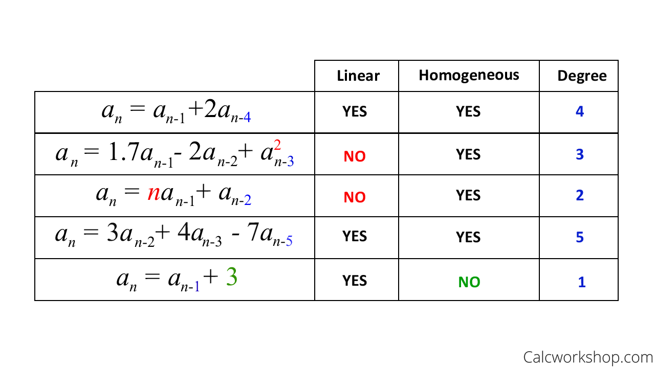
This table classifies five different recurrence relations. Notice that for a relation to be linear, homogeneous, and have constant coefficients, all terms must be of the form $c \cdot a_k$, where c is a constant.

Today, we are focusing on solving relations that are marked "YES" for both Linear and Homogeneous and have constant coefficients, like the first and fourth examples in the table.

The Characteristic Equation Method

The core idea is to guess that the solution is of the form $a_{n} = r^{n}$ for some non-zero constant $r$ . This is a geometric progression. Let's see what happens when we substitute this guess into a typical second-order recurrence:
$a_{n} = c_{1} a_{n - 1} + c_{2} a_{n - 2}$
Substituting our guess gives:
$r^{n} = c_{1} r^{n - 1} + c_{2} r^{n - 2}$
Since we assumed $r \neq = 0$ , we can divide the entire equation by the smallest power of $r$ , which is $r^{n - 2}$ :
$r^{2} = c_{1} r + c_{2}$
Rearranging gives us a simple quadratic equation:
$r^{2} - c_{1} r - c_{2} = 0$
This is called the characteristic equation of the recurrence relation. The roots of this polynomial are the key to finding the closed-form solution.

Case 1: Distinct Roots

Let's say we solve the characteristic equation and find two distinct real roots, $r_{1}$ and $r_{2}$ . This means both $a_{n} = r_{1}^{n}$ and $a_{n} = r_{2}^{n}$ are solutions. A key property of linear homogeneous relations (the "superposition principle") is that any linear combination of solutions is also a solution. Thus, the general solution is:
$a_{n} = A r_{1}^{n} + B r_{2}^{n}$
The constants $A$ and $B$ are determined by the initial conditions of the sequence (e.g., the values of $a_{0}$ and $a_{1}$ ).

Let's walk through an example. Find the closed form for $a_{n} = 5 a_{n - 1} - 6 a_{n - 2}$ with initial conditions $a_{0} = 1$ and $a_{1} = 1$ .

Characteristic Equation: $r^{2} - 5 r + 6 = 0$ .
Find the Roots: Factoring gives $(r - 2) (r - 3) = 0$ . The roots are $r_{1} = 2$ and $r_{2} = 3$ .
General Solution: Since the roots are distinct, the general form is $a_{n} = A \cdot 2^{n} + B \cdot 3^{n}$ .
Solve for Constants: We use the initial conditions to create a system of equations:
- For $n = 0$ : $a_{0} = 1 = A \cdot 2^{0} + B \cdot 3^{0} ⟹ 1 = A + B$
- For $n = 1$ : $a_{1} = 1 = A \cdot 2^{1} + B \cdot 3^{1} ⟹ 1 = 2 A + 3 B$
- Solving this system (e.g., by substituting $A = 1 - B$ into the second equation) gives $B = - 1$ and $A = 2$ .
Final Solution: $a_{n} = 2 \cdot 2^{n} - 1 \cdot 3^{n} = 2^{n + 1} - 3^{n}$ .

The following video provides an excellent, step-by-step tutorial on this exact process.

Discrete Math II - 8.2.2 Solving Second-Order Linear Homogeneous Recurrence Relations

This video by Kimberly Brehm provides a very clear, pedagogical walkthrough of solving a second-order linear homogeneous recurrence relation with distinct roots.

Watch the segments from the beginning and from the first two examples. The first example, starting at 0:45, is almost identical to the one we just did. The second example reinforces the method with different numbers and shows an alternative way to solve the system of equations.

For a concise, text-based summary of this method, the Art of Problem Solving Wiki is a great resource.

Characteristic polynomial - AoPS Wiki

This wiki page provides a compact definition of the characteristic polynomial for linear recurrences and a fully worked-out example.

Read the section on linear recurrences for a quick summary. Then, review the worked-out problem, which follows the same steps we just covered.

Case 2: Repeated Roots

What if the characteristic equation has a repeated root? For example, consider $a_{n} = 6 a_{n - 1} - 9 a_{n - 2}$ .
The characteristic equation is $r^{2} - 6 r + 9 = 0$ , which factors to $(r - 3)^{2} = 0$ . The only root is $r = 3$ , with a multiplicity of 2.

In this case, we can't form the solution as $A \cdot 3^{n} + B \cdot 3^{n}$ because that simplifies to $(A + B) 3^{n}$ , leaving us with only one constant to solve for, which isn't enough.

The rule for a repeated root $r_{1}$ of multiplicity $m$ is that the solution involves powers of $n$ . For a double root ( $m = 2$ ), the general solution is:
$a_{n} = (A + B n) r_{1}^{n}$
For our example with $r_{1} = 3$ , the solution is $a_{n} = (A + B n) 3^{n}$ . The constants $A$ and $B$ are found using the initial conditions, just as before.

The same video resource explains this modification very clearly.

Discrete Math II - 8.2.2 Solving Second-Order Linear Homogeneous Recurrence Relations

The second half of Kimberly Brehm's video is dedicated to handling cases with repeated roots.

Now, watch from this timestamp to the end. The video walks through two examples of finding closed-form solutions when the characteristic equation has a repeated root. Pay close attention to how the general form of the solution changes by including the n term.

Generalizing the Method

This method extends naturally to higher-order recurrences. A $k$ -th order recurrence will have a characteristic polynomial of degree $k$ . If all roots $r_{1}, \dots, r_{k}$ are distinct, the solution is $a_{n} = A_{1} r_{1}^{n} + \dots + A_{k} r_{k}^{n}$ . If a root has multiplicity, you introduce polynomial terms in $n$ .

The following resource formalizes this for any order $k$ .

Recurrence Relations

This document from the Canadian Mathematical Society provides a formal definition for higher-order relations.

Read the section titled "Linear Recurrence Relations of Order k". This section shows the general form of the solution for a polynomial with roots of varying multiplicities. You don't need to memorize it, but it's good to see the general pattern.

Practice Problems

It's time to put this method into practice. Your goal is to find the closed-form solution for each of the following recurrence relations. Follow the five-step process: find the characteristic equation, find the roots, write the general form, use the initial conditions to find the constants, and write the final solution.

These problems are taken from the CMS document. You can check your answers in the back of the PDF, but try your best to solve them on your own first!

Distinct Roots: Solve the recurrence relation $a_{n} + a_{n - 1} - 6 a_{n - 2} = 0$ for $n \geq 2$ , with $a_{0} = 7, a_{1} = 4$ .
(This corresponds to Exercise 5 in the PDF).
Repeated Roots: Solve the recurrence relation $a_{n} - 6 a_{n - 1} + 9 a_{n - 2} = 0$ for $n \geq 2$ , with $a_{0} = - 2, a_{1} = 6$ .
(This corresponds to Exercise 4 in the PDF).
A Challenge (Third-Order): Find $a_{n}$ if $a_{n} - 5 a_{n - 1} + 8 a_{n - 2} - 4 a_{n - 3} = 0$ for $n \geq 3$ , with $a_{0} = 0, a_{1} = 2, a_{2} = 4$ .
(This is Exercise 8. Hint: The characteristic polynomial is $r^{3} - 5 r^{2} + 8 r - 4 = 0$ . You will need to find the roots of this cubic. Try testing small integer values like 1, 2, -1, -2 to find a first root, then use polynomial division).

You can find the problems and their solutions here for reference after you've attempted them.

Recurrence Relations

This PDF contains the exercises and their worked-out solutions.

The problems are in the "Exercises" section. The solutions start on page 52, under the heading "Solutions and Answers".

Conclusion

Today you've added a crucial algebraic tool to your combinatorial arsenal. You learned to identify linear homogeneous recurrence relations with constant coefficients and solve them systematically using the characteristic equation method. We covered the two main cases: when the roots of the characteristic polynomial are distinct and when they are repeated. This process allows us to convert a recursive definition into a direct, closed-form formula, which is a massive leap in analytical power.

However, this method is limited. It doesn't work for non-homogeneous relations like the plane division problem ( $L_{n} = L_{n - 1} + n$ ), nor does it offer a way to handle more complex recurrences. In our next lesson, we will begin exploring an even more powerful and versatile tool: generating functions. We will see how to represent an entire infinite sequence as a single polynomial-like object, opening the door to solving a much wider class of recurrence relations and counting problems.

Recommended resources