Decision Trees and Feature Importance

1. What is a Decision Tree?

At its core, a decision tree is a model that predicts the value of a target variable by learning simple decision rules inferred from the data features. It's like a game of "20 Questions," where each question narrows down the possibilities until you arrive at a final answer.

The tree has a hierarchical structure:

• Root Node: The starting point, representing the entire dataset.
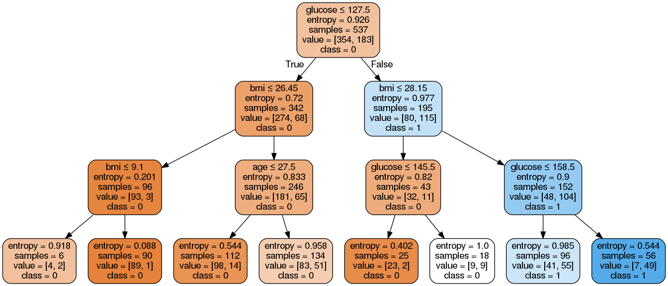
• Internal Nodes: These represent a "test" on a feature (e.g., "Is age < 54.5?").
• Branches: The outcomes of a test (e.g., "Yes" or "No"), leading to the next node.
• Leaf Nodes: The terminal nodes that represent the final decision or class label (e.g., "Has Heart Disease").

This structure makes decision trees highly interpretable, often called "white box" models, because you can follow the path of decisions for any given data point.

2. How a Decision Tree Learns: The Art of Splitting

The main challenge in building a decision tree is to figure out the best questions to ask at each node. How does the algorithm decide that "Is age < 54.5?" is a better first question than "Is cholesterol > 300?"

The answer lies in finding splits that make the resulting groups as "pure" or homogeneous as possible. A pure node would contain samples from only one class. The algorithm's goal is to select the feature and split value that results in the greatest reduction in impurity.

Two common metrics are used to measure impurity:

1. Gini Impurity: This measures the probability of incorrectly classifying a randomly chosen element in the dataset if it were randomly labeled according to the class distribution in that set. A Gini score of 0 means the node is perfectly pure (all samples belong to one class). A score of 0.5 (for a binary problem) means the node is maximally impure (a 50/50 split of classes). The formula is:
   $\text{Gini}=1-{\sum }_{i=1}^k(p_i{)}^2$
   where $p_i$ is the probability of an item being in class $i$.

2. Entropy: A concept from information theory that measures the level of disorder or uncertainty in a node. Like Gini, an entropy of 0 means the node is pure. The reduction in entropy is called Information Gain.

Scikit-learn uses Gini impurity by default, so we'll focus on that. The algorithm works as follows at each node:

1. Iterate through every feature.
2. For each feature, iterate through all possible split values.
3. Calculate the weighted average Gini impurity of the child nodes that would result from that split.
4. Choose the feature and split value that lead to the lowest weighted Gini impurity (i.e., the highest "Gini Gain" or impurity reduction).
5. Repeat this process recursively for each new child node until a stopping criterion is met (e.g., the node is pure, the tree reaches a maximum depth, or a node has too few samples to split).

3. Training a Decision Tree with Scikit-Learn

Now that you understand the theory, let's put it into practice with Python. Your experience with scikit-learn for logistic regression will be very useful here, as the workflow is almost identical.

We'll use the DecisionTreeClassifier from sklearn.tree.

Here is a consolidated code example based on that workflow. Notice how simple it is to train the model and make predictions.

import pandas as pd
from sklearn.model_selection import train_test_split
from sklearn.tree import DecisionTreeClassifier, plot_tree
import matplotlib.pyplot as plt




# Using a heart disease dataset for this example
# 1. Load Data
df = pd.read_csv('https://drive.google.com/uc?export=download&id=1wD8BDvD0nl6aO_qRbANX83vOAA6cvRTn')




# 2. Define Features (X) and Target (y)
X = df.drop('heart disease', axis=1)
y = df['heart disease']




# 3. Split Data
X_train, X_test, y_train, y_test = train_test_split(X, y, train_size=0.7, random_state=42)




# 4. Create and Fit the Model
# We'll set max_depth=3 to keep the tree small and interpretable
dt_classifier = DecisionTreeClassifier(max_depth=3, random_state=42)
dt_classifier.fit(X_train, y_train)




# 5. Evaluate the model
accuracy = dt_classifier.score(X_test, y_test)
print(f"Model accuracy on the test set: {accuracy:.2f}")




# 6. Visualize the Tree
plt.figure(figsize=(20,10))
plot_tree(dt_classifier, 
          feature_names=X.columns, 
          class_names=['No Disease', 'Disease'], 
          filled=True, 
          rounded=True)
plt.show()

If you run this code, you'll see a visualization of the trained tree. Each node shows the splitting condition, its Gini impurity, the number of samples in that node, and the class distribution.

A Note on Overfitting

If you don't set a max_depth or other constraints, a decision tree will keep splitting until every leaf is perfectly pure. This often results in a model that has memorized the training data and performs poorly on new, unseen data. This is called overfitting.

To prevent this, we use pre-pruning techniques by tuning hyperparameters like:

• max_depth: The maximum depth of the tree.
• min_samples_split: The minimum number of samples a node must have before it can be split.
• min_samples_leaf: The minimum number of samples required to be at a leaf node.

4. Explaining Feature Importance

This brings us to the second part of our learning goal. How do we quantify which features were most important in making predictions?

In a decision tree, a feature's importance is the total reduction in impurity it provides, summed up across all nodes where that feature is used for a split. The contributions are weighted by the number of samples in each node. Scikit-learn automatically calculates this for us and makes it available in the feature_importances_ attribute after the model is trained.

Let's add to our code to see the feature importances for our heart disease model.

# (Code from the previous block...)




# 7. Get Feature Importances
importances = dt_classifier.feature_importances_
feature_importance_df = pd.DataFrame({
    'feature': X.columns,
    'importance': importances
}).sort_values('importance', ascending=False)

print("\nFeature Importances:")
print(feature_importance_df)




# Output might look like this:
#
# Feature Importances:
#                      feature  importance
# 12                        ca    0.463391
# 2                         cp    0.222345
# 9                    thalach    0.133261
# 0                        age    0.054452
# 7                      oldpeak    0.050311
# ... and so on

This tells us that in our small tree, the 'ca' (number of major vessels colored by flourosopy) and 'cp' (chest pain type) features were the most decisive in splitting the data and reducing impurity.

Conclusion

Great job! You have now mastered a non-linear model that is both powerful and highly interpretable.

Key Takeaways:

• Decision Trees are flowchart-like models that classify data by making a series of decisions on features.
• They are built using a greedy, top-down approach, where each split is chosen to achieve the maximum reduction in impurity.
• Common impurity measures are Gini Impurity and Entropy.
• Feature Importance is calculated as the total impurity reduction a feature provides across all splits in the tree.
• Decision trees are prone to overfitting, which can be controlled by tuning hyperparameters like max_depth and min_samples_leaf.

In our next lesson, we will see how to overcome some of the limitations of single decision trees (like their tendency to overfit) by combining many of them into powerful ensemble models like Random Forests and Gradient Boosting.