Linear Regression: Implementation and Interpretation

1. What is Linear Regression?

At its heart, linear regression tries to model the relationship between a dependent variable (the value we want to predict, often called y) and one or more independent variables (our features, often called X). It does this by finding an equation for a straight line that best "fits" the data points.

You might remember the equation of a line from school:

$y=mx+b$

In machine learning, this is often written as:

$y={\beta }_{1}x+{\beta }_0$

Here:

• $y$ is the value we want to predict (e.g., house price).
• $x$ is our input feature (e.g., square footage of the house).
• ${\beta }_1$ is the coefficient or slope of the line. It determines how much $y$ changes when $x$ changes.
• ${\beta }_0$ is the intercept of the line. It's the value of $y$ when $x$ is zero.

The model's job is to find the optimal values for ${\beta }_1$ (the slope) and ${\beta }_0$ (the intercept) that result in a line that is closest to all the data points. This "best fit" line is the one that minimizes the total error between its predictions and the actual data points.

The Math Behind the "Best Fit"

How does the algorithm decide which line is "best"? It calculates the vertical distance (the error or residual) from each data point to the line, squares that distance, and adds them all up. This is called the Sum of Squared Errors (SSE) or Residual Sum of Squares (RSS). The line with the minimum possible SSE is the "best fit" line.

To give you a better intuition for this error function, let's watch another short clip.

The process of finding the minimum of this error function is a core concept in machine learning called optimization. While the underlying calculus involves partial derivatives and gradient descent, you don't need to master it to use the model. The libraries we use handle it for us.

2. Implementing Linear Regression with Scikit-Learn

Now for the practical part. Your background in Python will be very useful here. We will use scikit-learn, the most popular library for general-purpose machine learning in Python, to build our model.

The following reading provides a clear, step-by-step guide to implementing simple linear regression.

Let's consolidate what you've just read into a complete code example. We'll use the home price prediction scenario from the first video.

import pandas as pd
from sklearn.model_selection import train_test_split
from sklearn.linear_model import LinearRegression




# 1. Load and Prepare Data
# In a real project, you'd load from a file. Here we create it directly.
data = {'area': [2600, 3000, 3200, 3600, 4000],
        'price': [550000, 565000, 610000, 680000, 725000]}
df = pd.DataFrame(data)




# Separate features (X) and target (y)
X = df[['area']] # Features must be a 2D array or DataFrame
y = df['price']




# Split data (as learned in the previous lesson)
X_train, X_test, y_train, y_test = train_test_split(X, y, test_size=0.2, random_state=42)




# 2. Create and Fit the Model
# Create an instance of the LinearRegression model
model = LinearRegression()




# Fit the model to the training data. This is where the model "learns".
model.fit(X_train, y_train)




# 3. Get Results (The Coefficients)
# The model has now calculated the best intercept and coefficient.
intercept = model.intercept_
coefficient = model.coef_[0] # .coef_ is an array, we get the first element

print(f"Intercept (b): {intercept:.2f}")
print(f"Coefficient (m): {coefficient:.2f}")




# 4. Make Predictions
# Predict the price for a house with 3300 sq ft
predicted_price = model.predict([[3300]])
print(f"Predicted price for 3300 sq ft: ${predicted_price[0]:.2f}")




# You can also use the formula directly:
manual_prediction = coefficient * 3300 + intercept
print(f"Manual calculation for 3300 sq ft: ${manual_prediction:.2f}")

3. Interpreting the Coefficients

Getting the numbers for the intercept and coefficient is only half the job. The real value comes from understanding what they mean.

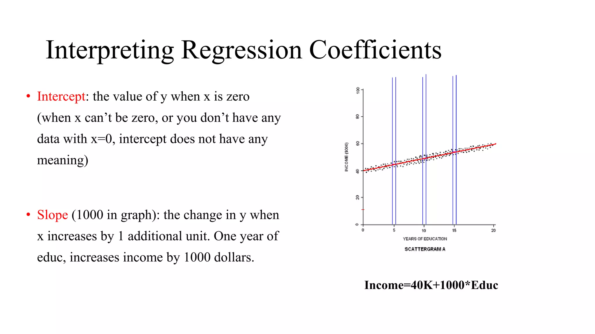
To formalize this understanding, please read the following brief explanation.

Let's apply this to our home price example. If our model returned:

• Intercept (${\beta }_0$): 180616.44
• Coefficient (${\beta }_1$): 135.79

Here is the correct interpretation:

• Intercept: The predicted price of a house with an area of 0 square feet is approximately $180,616. In many real-world scenarios like this one, the intercept is not practically meaningful on its own but serves as the necessary starting point for the line.
• Coefficient: For every one-unit increase in area (i.e., for each additional square foot), the model predicts that the house price will increase by approximately $135.79. This value quantifies the relationship between area and price that the model has learned from the data.

What about Multiple Features?

Simple linear regression uses one feature. More often, you'll use multiple linear regression with many features (e.g., area, number of bedrooms, age of house). The equation expands:

$\text{price}={\beta }_0+{\beta }_1\cdot \text{area}+{\beta }_2\cdot \text{bedrooms}+{\beta }_3\cdot \text{age}$

The interpretation is similar but with an important addition:

• ${\beta }_1$: The predicted change in price for a one-unit increase in area, holding the number of bedrooms and age constant.
• ${\beta }_2$: The predicted change in price for one additional bedroom, holding the area and age constant.

Each coefficient tells you the independent contribution of its feature to the prediction.

Conclusion

Congratulations on building and interpreting your first machine learning model! This is a fundamental skill for any AI developer.

Key Takeaways:

• Linear regression models the linear relationship between features and a continuous target variable by finding a "best fit" line.
• This line is found by minimizing the Sum of Squared Errors (SSE) between the model's predictions and the actual data.
• In scikit-learn, you use LinearRegression().fit(X_train, y_train) to train the model.
• The intercept (.intercept_) is the predicted value of the target when all features are zero.
• The coefficient (.coef_) tells you how much the target is expected to change for a one-unit change in a feature, holding all other features constant.

Now that you can predict continuous values like price, what if you need to predict categories, such as 'spam' or 'not spam'? For that, we need a different kind of model. In the next lesson, we will explore logistic regression for binary classification tasks.