Confusion Matrix & Performance Metrics

1. The Limits of Accuracy

In many classification problems, simply measuring accuracy (the percentage of correct predictions) can be dangerously misleading.

Imagine you're building a model to detect a rare disease that affects only 1% of the population. A lazy model that predicts "no disease" for every single person would have 99% accuracy! It's technically correct most of the time, but it's completely useless because it fails to identify any of the sick patients, which is the entire point of the model.

This is a classic example of an imbalanced dataset, where one class is far more frequent than the other. In such cases, and many others, we need a better way to understand a model's performance.

To explore this further, let's start with a quick read that highlights the limitations of accuracy.

2. The Confusion Matrix: A Deeper Look at Performance

The foundation for better evaluation is the confusion matrix. It's a table that breaks down a model's predictions and compares them to the actual ground truth. This allows us to see not just how many predictions were wrong, but also what kind of errors the model is making.

For a binary classification problem (e.g., "spam" vs. "not spam"), the confusion matrix has four components:

• True Positives (TP): The model correctly predicted the positive class. (e.g., correctly identified a spam email as "spam").
• True Negatives (TN): The model correctly predicted the negative class. (e.g., correctly identified a normal email as "not spam").
• False Positives (FP): The model incorrectly predicted the positive class. (e.g., marked a normal email as "spam"). This is also known as a Type I Error.
• False Negatives (FN): The model incorrectly predicted the negative class. (e.g., let a spam email into the inbox, marking it as "not spam"). This is also known as a Type II Error.

The following video provides an excellent, intuitive explanation of these terms and how they fit together in a confusion matrix.

Here is a visual representation of a confusion matrix. The diagonal elements (top-left to bottom-right) represent correct predictions, while the off-diagonal elements represent errors.

3. Precision, Recall, and the F1-Score

Now that we have the counts of TP, TN, FP, and FN, we can calculate more meaningful metrics: Precision, Recall, and the F1-Score.

Precision: How Trustworthy Are the Positive Predictions?

Precision answers the question: "Of all the instances the model predicted as positive, how many were actually positive?"

$\text{Precision}=\frac{\text{TP}}{\text{TP}+\text{FP}}$

• When is it important? High precision is critical when the cost of a False Positive (FP) is high.
  • Spam Detection: You don't want important emails (e.g., a job offer) to be incorrectly marked as spam.
  • Legal System: You don't want to convict an innocent person.

Recall: How Many Positives Did We Find?

Recall (also known as Sensitivity or True Positive Rate) answers the question: "Of all the actual positive instances, how many did the model successfully identify?"

$\text{Recall}=\frac{\text{TP}}{\text{TP}+\text{FN}}$

• When is it important? High recall is critical when the cost of a False Negative (FN) is high.
  • Medical Diagnosis: You absolutely do not want to miss a case of a serious illness.
  • Fraud Detection: You want to catch as many fraudulent transactions as possible, even if it means flagging a few legitimate ones for review.

The Precision-Recall Trade-off

You will often find a trade-off between precision and recall. If you tune your model to be very strict about predicting positives, you will have fewer FPs (higher precision) but you might miss some real positives, leading to more FNs (lower recall). Conversely, if you loosen the criteria, you'll find more of the true positives (higher recall) but likely at the cost of mislabeling more negatives as positive (lower precision).

F1-Score: A Single Metric to Rule Them All

Since you often need to balance precision and recall, the F1-Score was created. It is the harmonic mean of precision and recall.

$\text{F1-Score}=2\times \frac{\text{Precision}\times \text{Recall}}{\text{Precision}+\text{Recall}}$

The F1-score provides a single number that reflects this balance. It's generally more useful than accuracy on imbalanced datasets because it takes both false positives and false negatives into account. A high F1-score requires both high precision and high recall.

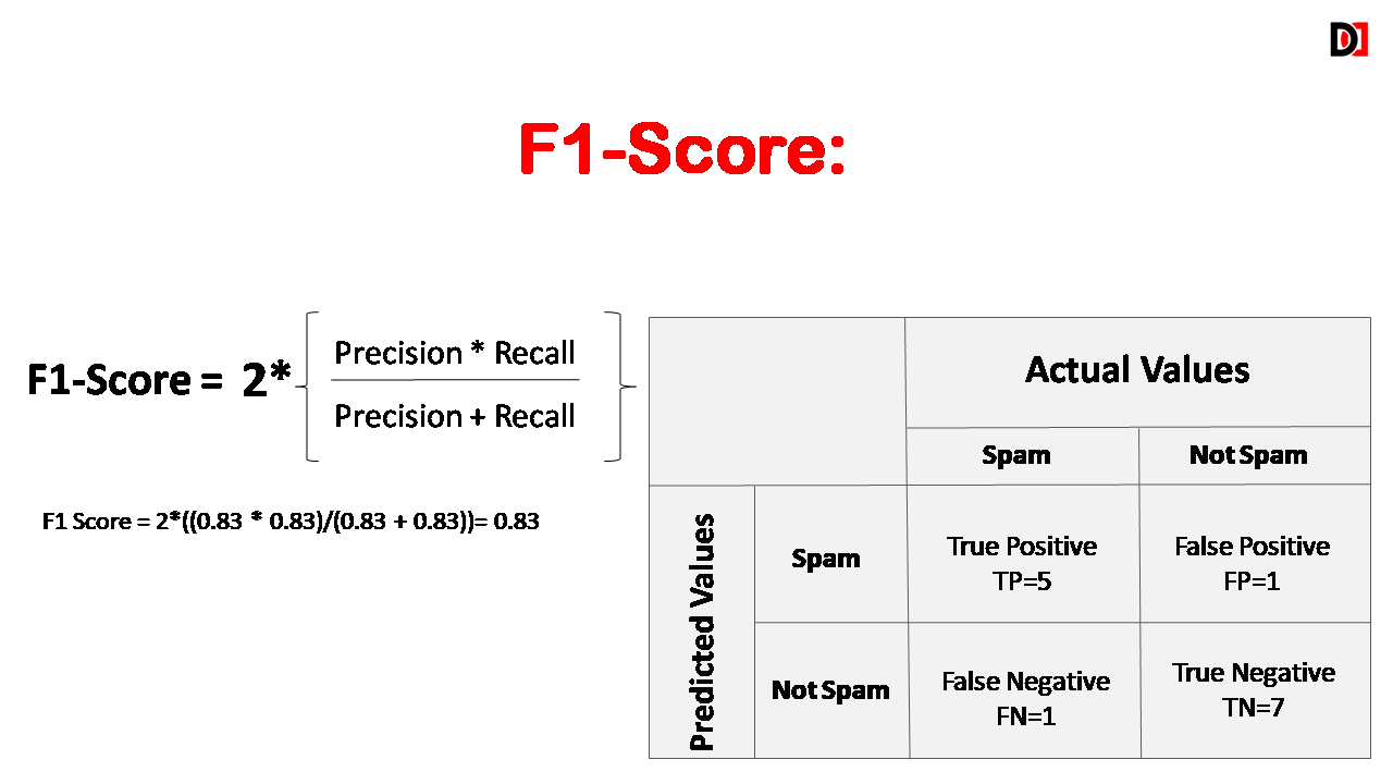
Let's return to the video to see these concepts explained with the same clear example.

4. Putting It All Together with Scikit-Learn

Manually calculating these metrics is great for understanding, but in practice, you'll use libraries like scikit-learn to do it for you. The two key functions are:

1. confusion_matrix(): Generates the matrix itself.
2. classification_report(): Generates a text report showing precision, recall, and F1-score for each class.

Let's see how to implement this in Python. We'll use the Random Forest model from our previous lesson.

import numpy as np
from sklearn.ensemble import RandomForestClassifier
from sklearn.model_selection import train_test_split
from sklearn.datasets import make_classification



# Import the evaluation metrics
from sklearn.metrics import confusion_matrix, classification_report
import seaborn as sns
import matplotlib.pyplot as plt




# Generate a sample dataset (same as last lesson)
# We make it slightly imbalanced to better see the value of these metrics
X, y = make_classification(
    n_samples=1000, 
    n_features=20, 
    n_informative=10, 
    n_redundant=5, 
    n_classes=2,
    weights=[0.9, 0.1], # 90% class 0, 10% class 1
    random_state=42
)




# Split data
X_train, X_test, y_train, y_test = train_test_split(X, y, test_size=0.3, random_state=42, stratify=y)




# Create and fit the Random Forest model
rf_classifier = RandomForestClassifier(n_estimators=100, random_state=42)
rf_classifier.fit(X_train, y_train)




# Make predictions
y_pred = rf_classifier.predict(X_test)




# 1. Generate and print the confusion matrix
cm = confusion_matrix(y_test, y_pred)
print("Confusion Matrix:")
print(cm)
print("-" * 30)




# Optional: Visualize the confusion matrix
sns.heatmap(cm, annot=True, fmt='d', cmap='Blues')
plt.ylabel('Actual')
plt.xlabel('Predicted')
plt.title('Confusion Matrix')
plt.show()




# 2. Generate and print the classification report
report = classification_report(y_test, y_pred, target_names=['Class 0', 'Class 1'])
print("Classification Report:")
print(report)

When you run this code, you'll get two outputs.

First, the confusion matrix:

Confusion Matrix:
[[265   5]
 [ 16  14]]

Note: In scikit-learn's confusion_matrix, the rows represent the actual classes and the columns represent the predicted classes.

• TN = 265: 265 instances of 'Class 0' were correctly predicted.
• FP = 5: 5 instances of 'Class 0' were incorrectly predicted as 'Class 1'.
• FN = 16: 16 instances of 'Class 1' were incorrectly predicted as 'Class 0'.
• TP = 14: 14 instances of 'Class 1' were correctly predicted.

Second, the classification report, which neatly summarizes all the metrics:

Classification Report:
              precision    recall  f1-score   support

     Class 0       0.94      0.98      0.96       270
     Class 1       0.74      0.47      0.57        30

    accuracy                           0.93       300
   macro avg       0.84      0.72      0.77       300
weighted avg       0.92      0.93      0.92       300

This report is incredibly useful. For our minority class ('Class 1'), we can see the model has decent precision (0.74) but poor recall (0.47), meaning when it predicts 'Class 1' it's right 74% of the time, but it's only finding 47% of all the actual 'Class 1' instances. The F1-score (0.57) reflects this imbalance.

The following resources provide a final review of these concepts and their scikit-learn implementation.

Conclusion

In this lesson, you've moved beyond simple accuracy and learned to evaluate classification models with a professional, nuanced perspective.

Key Takeaways:

• Accuracy is not enough, especially when dealing with imbalanced datasets or when the costs of different errors vary.
• The Confusion Matrix is a fundamental tool that breaks down a model's performance into True/False Positives and True/False Negatives.
• Precision measures the quality of positive predictions (low FP is key), while Recall measures the completeness of positive predictions (low FN is key).
• The F1-Score is the harmonic mean of precision and recall, providing a single, balanced metric to compare models.
• scikit-learn provides easy-to-use functions like confusion_matrix and classification_report to automate this analysis.

In our next lesson, we will continue our journey into model evaluation by exploring the ROC curve and AUC metric. These tools help us visualize the trade-off between a model's true positive rate and false positive rate, allowing us to choose the optimal classification threshold for our specific problem.