Electron-Hole Pair Hamiltonian Formulation

Introduction

In the previous lessons, we built a strong phenomenological understanding of excitons by exploring the two limiting cases: the delocalized Wannier-Mott exciton, described by an effective mass hydrogen model, and the localized Frenkel exciton, described by a tight-binding model. While useful, these are separate pictures. To build a unified and more powerful theory, we must go deeper.

Today, we transition from these models to a fundamental, many-body description. Our learning outcome is to formulate the electron-hole pair Hamiltonian using second quantization creation and annihilation operators. This formalism is the language of modern condensed matter theory and will be our primary tool for the rest of the course. You'll find the methods here analogous to those used in quantum field theory, but applied to the many-electron system of a solid.

By the end of this lesson, you will understand how to construct the complete Hamiltonian for a semiconductor and isolate the terms that describe the dynamics of an interacting electron-hole pair. This sets the stage for our next lesson, where we will solve this Hamiltonian to find the exciton states.

The Many-Electron Hamiltonian in Second Quantization

Let's begin by constructing the Hamiltonian for all interacting electrons in a crystal. The general form consists of three parts: the kinetic energy of the electrons, their potential energy in the periodic field of the atomic nuclei, and the pairwise Coulomb interaction between electrons.

As the video shows, a general many-electron Hamiltonian can be written as $H=H_0+H_{ee}$.

• $H_0$: The Single-Particle Part. This includes the electron kinetic energy and the interaction with the static, periodic potential of the ion lattice.
• $H_{ee}$: The Electron-Electron Interaction. This is the two-body term representing the Coulomb repulsion between every pair of electrons.

To make this concrete for a crystal, we use the basis of Bloch states, $|n,\mathbf{k}⟩$, which are the eigenstates of the single-particle problem. Here, $n$ is the band index (e.g., valence or conduction) and $\mathbf{k}$ is the crystal momentum. Let's denote the creation and annihilation operators for an electron in this state as $c_{n,\mathbf{k}}^{†}$ and $c_{n,\mathbf{k}}$, respectively. They obey the standard fermionic anti-commutation relations:

In this basis, the Hamiltonian takes the following form:

1. Single-Particle Hamiltonian $H_0$: Since the Bloch states diagonalize the single-particle part of the problem, $H_0$ is simply:

   $$H_0=\sum _{n,\mathbf{k}}{E}_n(\mathbf{k})c_{n,\mathbf{k}}^{†}{c}_{n,\mathbf{k}}$$

   Here, $E_n(\mathbf{k})$ is the energy of an electron in band $n$ with momentum $\mathbf{k}$—this is the electronic band structure of the material.

2. Electron-Electron Interaction $H_{ee}$: This term describes how electrons scatter off each other. It involves four operators, corresponding to annihilating two electrons in initial states and creating two in final states.

   $$H_{ee}=\frac{1}{2}\sum _{\begin{array}{c}{\mathbf{k}}_1,{\mathbf{k}}_2,\mathbf{q}\\ n_1,n_2,n_3,n_4\end{array}}{V}_{n_1,n_2,n_3,n_4}({\mathbf{k}}_1,{\mathbf{k}}_2,\mathbf{q})c_{n_1,{\mathbf{k}}_1+\mathbf{q}}^{†}{c}_{n_2,{\mathbf{k}}_2-\mathbf{q}}^{†}{c}_{n_3,{\mathbf{k}}_2}{c}_{n_4,{\mathbf{k}}_1}$$

   The term $V_{n_1,n_2,n_3,n_4}({\mathbf{k}}_1,{\mathbf{k}}_2,\mathbf{q})$ is the Coulomb matrix element, which depends on the overlap of the four Bloch wavefunctions involved. The sum is over all momenta and bands, and the factor of $\frac{1}{2}$ prevents double counting. The momentum $\mathbf{q}$ represents the momentum transfer during the collision.

The full Hamiltonian $H=H_0+H_{ee}$ is the exact (within the Born-Oppenheimer approximation) description of the electronic system. Our goal now is to see what this Hamiltonian looks like when we consider a single electron excited from a valence band to a conduction band.

The Hole Formalism

To talk about excitons, we need to describe not just the excited electron but also the vacancy it leaves behind. The key insight is to treat this vacancy—the hole—as a particle in its own right.

Let's formalize this. We first define the semiconductor's ground state, $|G⟩$, as the state where all valence bands are completely filled with electrons and all conduction bands are completely empty. This is our "vacuum" for excitations.

• For any conduction band state $|c,\mathbf{k}⟩$, $c_{c,\mathbf{k}}|G⟩=0$ (no electrons to annihilate).
• For any valence band state $|v,\mathbf{k}⟩$, $c_{v,\mathbf{k}}^{†}|G⟩=0$ (Pauli exclusion prevents adding another electron).

An exciton is created by moving an electron from a valence band state $|v,{\mathbf{k}}_h⟩$ to a conduction band state $|c,{\mathbf{k}}_e⟩$. The state of the system is $c_{c,{\mathbf{k}}_e}^{†}{c}_{v,{\mathbf{k}}_h}|G⟩$.

Notice that annihilating an electron with momentum ${\mathbf{k}}_h$ in the valence band creates the absence of an electron, which we identify as the hole. This suggests the following definitions for hole creation ($h^{†}$) and annihilation ($h$) operators:

• Hole Creation: Creating a hole with momentum $-{\mathbf{k}}_h$ and in band $v$ is equivalent to annihilating an electron in state $|v,{\mathbf{k}}_h⟩$.
  $h_{v,-{\mathbf{k}}_h}^{†}\equiv c_{v,{\mathbf{k}}_h}$
• Hole Annihilation: Annihilating a hole with momentum $-{\mathbf{k}}_h$ is equivalent to creating an electron in state $|v,{\mathbf{k}}_h⟩$.
  $h_{v,-{\mathbf{k}}_h}\equiv c_{v,{\mathbf{k}}_h}^{†}$

The choice of $-{\mathbf{k}}_h$ for the hole momentum is a convention that simplifies the equations of motion, ensuring that the total momentum of the electron-hole pair is $\mathbf{K}={\mathbf{k}}_e+{\mathbf{k}}_h$. The hole inherits the properties of the missing electron but with opposite charge and momentum.

The Effective Electron-Hole Hamiltonian

With the hole operators defined, we can now rewrite the full Hamiltonian $H=H_0+H_{ee}$ to describe the interactions within the subspace of single electron-hole pair states. For simplicity, we consider a two-band model with one conduction band ($c$) and one valence band ($v$).

The derivation is quite involved, as it requires systematically applying the Hamiltonian to a general one-electron-one-hole state and evaluating the matrix elements. This process is detailed in Section 3.5 of the resource LINK. Here, we will focus on the structure of the resulting effective Hamiltonian, which contains three main types of terms:

1. Single-Particle Energies: These terms come from $H_0$ and describe the energy of the electron and hole as if they were non-interacting. The total energy is the energy required to create the pair:
   $H_{\text{kin}}={\sum }_{{\mathbf{k}}_e}{E}_c({\mathbf{k}}_e)c_{c,{\mathbf{k}}_e}^{†}{c}_{c,{\mathbf{k}}_e}+{\sum }_{{\mathbf{k}}_h}(-E_v(-{\mathbf{k}}_h))h_{v,{\mathbf{k}}_h}^{†}{h}_{v,{\mathbf{k}}_h}$
   The energy of the hole is $-E_v(-{\mathbf{k}}_h)$, which is positive since valence band energies are negative relative to the Fermi level. Often, we measure energies from the band edges, so this becomes $E_g+\frac{{\hslash }^2{k}_e^2}{2m_e^{\ast }}+\frac{{\hslash }^2{k}_h^2}{2m_h^{\ast }}$.

2. Direct Coulomb Interaction: This is the most intuitive interaction term. It arises from $H_{ee}$ and describes the scattering of an electron and a hole due to their Coulomb attraction.

   $$H_{\text{direct}}=-\sum _{\begin{array}{c}{\mathbf{k}}_e,{\mathbf{k}}_h,\mathbf{q}\end{array}}V(\mathbf{q})c_{c,{\mathbf{k}}_e-\mathbf{q}}^{†}{h}_{v,{\mathbf{k}}_h+\mathbf{q}}^{†}{h}_{v,{\mathbf{k}}_h}{c}_{c,{\mathbf{k}}_e}$$

   Here, $V(\mathbf{q})$ is the Fourier transform of the screened Coulomb potential $e^2/(ϵ|{\mathbf{r}}_1-{\mathbf{r}}_2|)$. An electron at ${\mathbf{k}}_e$ and hole at ${\mathbf{k}}_h$ scatter, exchanging momentum $\mathbf{q}$, into new states ${\mathbf{k}}_e-\mathbf{q}$ and ${\mathbf{k}}_h+\mathbf{q}$. The negative sign is crucial: it reflects the attraction between the electron (negative charge) and the hole (positive charge).

3. Exchange Coulomb Interaction: This is a purely quantum mechanical effect arising from the indistinguishability of electrons and the Pauli exclusion principle. It corresponds to the virtual annihilation of the electron-hole pair and subsequent recreation.

   $$H_{\text{exchange}}=\sum _{\begin{array}{c}{\mathbf{k}}_e,{\mathbf{k}}_h,\mathbf{K}\end{array}}U(\dots )c_{c,{\mathbf{k}}_e}^{†}{h}_{v,\mathbf{K}-{\mathbf{k}}_e}^{†}{h}_{v,\mathbf{K}-{\mathbf{k}}_h}{c}_{c,{\mathbf{k}}_h}$$

   Here, $U(\dots )$ is the exchange matrix element. This term couples pairs with the same total momentum $\mathbf{K}={\mathbf{k}}_e+{\mathbf{k}}_h$. It is typically short-ranged and repulsive, and is responsible for the fine-structure splitting of exciton states (e.g., into singlets and triplets), a topic we will explore in detail later.

These interactions can be visualized using diagrams, which may be familiar from your QFT and advanced QM courses.

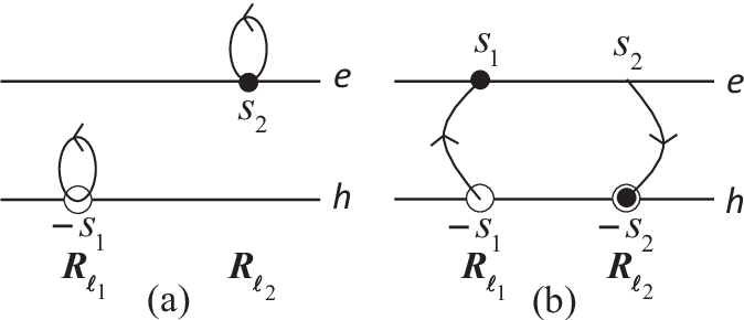
The diagram on the right (b) illustrates the direct Coulomb term. The electron and hole propagate, exchange momentum via the Coulomb interaction, and continue propagating in their new states.

Combining all parts, the effective Hamiltonian for the electron-hole system is:

This operator contains the full physics of the interacting electron-hole pair.

Conclusion

In this lesson, we have made a significant leap from phenomenological models to a fundamental many-body framework.

Key Takeaways:

• The Hamiltonian for a semiconductor can be written in second quantization using creation/annihilation operators for electrons in Bloch states.
• An electronic vacancy in a filled valence band can be treated as a quasiparticle—a hole—with positive charge and its own fermionic creation/annihilation operators.
• By restricting the full many-electron Hamiltonian to the subspace containing one electron-hole pair, we derived an effective Hamiltonian.
• This effective Hamiltonian includes:
  1. The kinetic energies of the electron and hole.
  2. An attractive direct Coulomb term describing their scattering.
  3. A repulsive exchange Coulomb term arising from particle indistinguishability.

Preview of the Next Lesson

We have successfully formulated the Hamiltonian that governs the exciton. The next logical step is to find its eigenstates and eigenvalues. Solving the Schrödinger equation associated with our $H_{\text{eff}}$ leads to a famous and powerful integral equation known as the Bethe-Salpeter Equation (BSE). In the next lesson, we will describe the structure of the BSE and show how it provides a complete description of the exciton's wavefunction, binding energy, and optical properties.