Exciton-Polaritons: Dispersion in Strong Coupling

Hello! Welcome to the final lesson in our module on the optical properties of excitons.

In our previous lessons, we treated light as a weak perturbation that causes transitions to excitonic states. This picture, governed by Fermi's golden rule, is what we call the weak-coupling regime. It successfully explains absorption spectra, including the selection rules we just derived. But what happens if the interaction between light and excitons becomes so strong that they can no longer be considered separate entities?

Today, we will answer that question by exploring the strong-coupling regime. Our goal is to introduce the concept of exciton-polaritons and derive the polariton dispersion relation. We will see that when light-matter coupling is dominant, the true elementary excitations of the system are no longer photons or excitons, but new hybrid quasiparticles called exciton-polaritons.

1. From Weak to Strong Coupling: The Polariton Concept

In the weak-coupling regime, a photon creates an exciton which then lives for some time before decaying (e.g., by emitting another photon). The processes are distinct. In the strong-coupling regime, the energy exchange between the exciton and the photon is so rapid that it's more accurate to say the energy exists as a coherent superposition of both.

This is typically achieved by placing a semiconductor quantum well (which hosts the excitons) inside a microcavity formed by two highly reflective Bragg mirrors. The cavity confines photons, creating a discrete set of photon modes that can interact strongly with the excitons in the well.

The new quasiparticle that emerges is the exciton-polariton: part-exciton, part-photon.

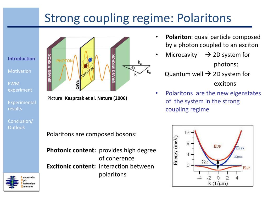
Strong Coupling Regime: Polaritons — This image provides a great conceptual overview. On the left is the physical system: an exciton in a quantum well interacting with a photon confined in a microcavity. On the right is the key result: the original, uncoupled exciton and photon dispersion curves (dashed) are replaced by two new curves for the Upper Polariton (UP) and Lower Polariton (LP), a phenomenon known as anti-crossing.

This mixing of properties has profound consequences:

The photonic component gives polaritons a very small effective mass and a finite lifetime due to leakage through the cavity mirrors. This allows us to probe the polaritons inside the cavity by measuring the light that escapes.
The excitonic component gives polaritons the ability to interact with each other, a crucial ingredient for observing many-body phenomena like Bose-Einstein condensation, which is one of your stated interests.

2. A Coupled Oscillator Model

At its core, the interaction between a single-mode cavity photon and a single exciton mode at the same momentum $k$ can be modeled as two coupled harmonic oscillators. Given your physics background, you'll recognize this classic problem.

Let $E_{e x c} (k)$ be the exciton energy and $E_{c a v} (k)$ be the cavity photon energy. If they are uncoupled, these are the system's energy levels. If we introduce a coupling energy, $g_{0}$ , the Hamiltonian for a given $k$ in the basis of single-excitation states ${∣ 1_{e x c}, 0_{p h} ⟩, ∣ 0_{e x c}, 1_{p h} ⟩}$ takes the form of a simple 2x2 matrix:

H^_{k} = (E_{e x c} (k) g_{0} g_{0} E_{c a v} (k))

Finding the eigenvalues of this matrix will give us the new energy levels of the coupled system. This is precisely what we will do now in a more formal second-quantized language.

3. The Polariton Hamiltonian and its Diagonalization

To formalize this, we write the Hamiltonian for the entire system of excitons and cavity photons. The following document presents this with excellent clarity.

Dynamic condensation of exciton-polaritons

The review paper 'Dynamic condensation of exciton-polaritons' by Deng, Haug, and Yamamoto provides a concise and rigorous derivation of the polariton dispersion. We will focus on the section that sets up and solves the problem.

Please read Section II.C.1, 'The Hamiltonian' (page 3 of the PDF). Pay close attention to Equation 11, which presents the Hamiltonian in second quantization form. Identify the terms corresponding to free photons, free excitons, and their interaction.

As you've just read, the Hamiltonian (using the rotating wave approximation, which is valid here) is:

H^= k \sum E_{c a v} (k) a^_{k}^{†} a^_{k} + k \sum E_{e x c} (k) b^_{k}^{†} b^_{k} + k \sum g_{0} (a^_{k}^{†} b^_{k} + a^_{k} b^_{k}^{†})

Here, $a^_{k}^{†}$ creates a cavity photon with in-plane momentum $k$ , and $b^_{k}^{†}$ creates an exciton with the same momentum. The coupling term $g_{0} (a^_{k}^{†} b^_{k} + h . c .)$ explicitly describes the process of annihilating an exciton to create a photon, and vice versa.

The new eigenstates, the polaritons, are found by diagonalizing this Hamiltonian. This is achieved through a canonical transformation (often called a Hopfield-Bogoliubov transformation) that defines new bosonic operators $P^_{k}$ and $Q^_{k}$ as linear combinations of the old ones:

P^_{k} = X_{k} b^_{k} + C_{k} a^_{k} (Lower Polariton)

Q^_{k} = - C_{k} b^_{k} + X_{k} a^_{k} (Upper Polariton)

The coefficients $X_{k}$ and $C_{k}$ are the Hopfield coefficients, which represent the excitonic and photonic fractions of the new polariton states, respectively, with $∣ X_{k} ∣^{2} + ∣ C_{k} ∣^{2} = 1$ .

Finding the eigenvalues of the 2x2 Hamiltonian matrix we discussed earlier yields the energies of the lower and upper polariton branches.

4. The Polariton Dispersion Relation

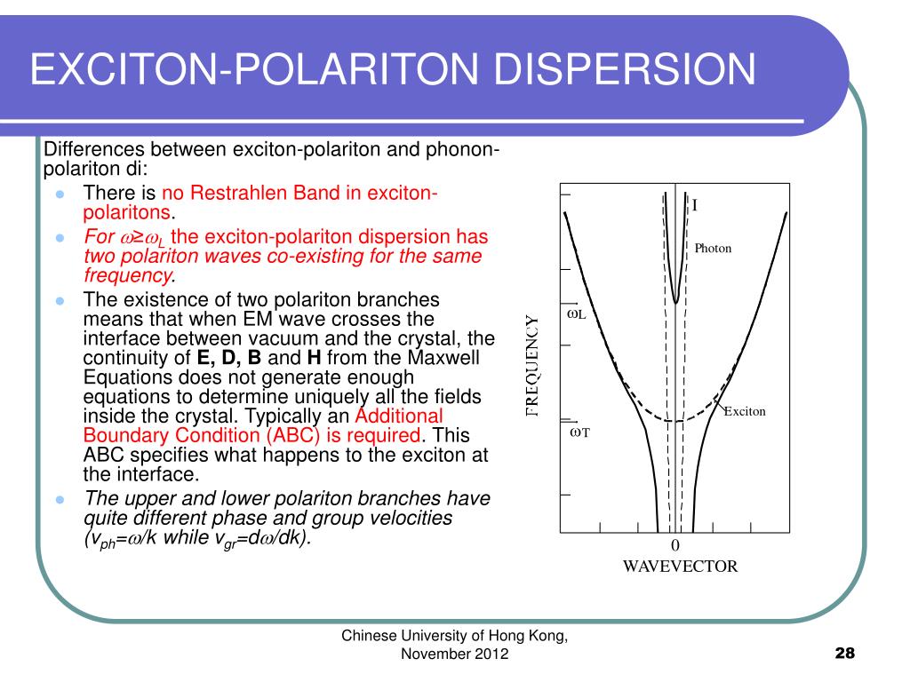
The diagonalization procedure yields the following energies for the two polariton branches:

E_{L P, U P} (k) = \frac{E _{e x c} ( k ) + E _{c a v} ( k )}{2} \pm \frac{1}{2} (E_{e x c} (k) - E_{c a v} (k))^{2} + 4 g_{0}^{2}

This equation is the central result of our lesson. It describes the energy-momentum relationship for the exciton-polaritons.

Let's analyze its structure:

The term inside the square root is composed of two parts: the energy detuning between the exciton and photon, $δ (k) = E_{e x c} (k) - E_{c a v} (k)$ , and the coupling energy $2 g_{0}$ .
At resonance ( $δ (k) = 0$ ), the two branches are separated by a minimum energy gap of $E_{U P} - E_{L P} = 2 g_{0}$ . This gap is known as the Rabi splitting.
Far from resonance ( $∣ δ (k) ∣ ≫ 2 g_{0}$ ), the square root approaches $∣ δ (k) ∣$ , and the polariton energies converge to the uncoupled exciton and photon energies.

This characteristic behavior is called anti-crossing and is the definitive signature of the strong-coupling regime.

Exciton-Polariton Dispersion Diagram and Key Characteristics — This dispersion diagram clearly illustrates the anti-crossing. The uncoupled photon and exciton dispersions (dashed lines) would cross, but the strong interaction forces them apart into the upper and lower polariton branches (solid lines). The minimum separation at resonance is the Rabi splitting.

5. The Strong-Coupling Condition and Polariton Properties

For the polariton picture to be valid, the coherent energy exchange between the exciton and photon must occur faster than either particle can decay or dephase. Let $γ_{c a v}$ and $γ_{e x c}$ be the total decay/broadening rates of the cavity and exciton, respectively. Strong coupling is achieved when:

g_{0} > \frac{γ _{c a v} + γ _{e x c}}{4}

This condition ensures that at least one full Rabi oscillation (energy swapping from exciton to photon and back) can occur before the coherence is lost. If this condition is not met, the system is in the weak-coupling regime, and the emission is simply modified by the cavity (an effect known as the Purcell effect).

To explore the consequences of this model, please continue with the same resource.

Dynamic condensation of exciton-polaritons

Now let's examine the consequences of this dispersion relation, particularly the polariton effective mass and the condition for strong coupling.

Please read Section II.C.2, 'Polariton dispersion and effective mass,' and Section II.C.3, 'Polariton decay' (pages 3-4 of the PDF). Focus on: The definition of the Rabi splitting (normal-mode splitting). The expression for the polariton effective mass (Eqs. 20-21) and the key result that the lower polariton mass can be extremely small near k=0. The strong-coupling criterion discussed in relation to the decay rates (page 4).

As you've seen, one of the most important consequences of polariton formation is the nature of the lower polariton branch. Because the photon dispersion is very steep (low effective mass, $m_{c a v} \approx 1 0^{- 5} m_{e}$ ) while the exciton dispersion is flat (high effective mass, $m_{e x c} \approx 0.5 m_{e}$ ), their mixture has unique properties. Near $k = 0$ , the lower polariton is mostly photon-like and inherits a very small effective mass: $m_{L P} \approx m_{c a v} /∣ C_{k} ∣^{2}$ . This is several orders of magnitude smaller than the free exciton mass and has major implications for achieving Bose-Einstein condensation at high temperatures.

Test your understanding!

Consider a system at zero detuning, so $E_{e x c} (k = 0) = E_{c a v} (k = 0)$ . What is the excitonic fraction, $∣ X_{k} ∣^{2}$ , and photonic fraction, $∣ C_{k} ∣^{2}$ , for both the lower and upper polaritons at $k = 0$ ? How does this change for the lower polariton if we tune the cavity to have a large positive detuning, $δ (0) = E_{c a v} (0) - E_{e x c} (0) ≫ g_{0}$ ?

Show answer

At zero detuning ( $δ (k) = 0$ ), the Hopfield coefficients simplify to $∣ X_{k} ∣^{2} = ∣ C_{k} ∣^{2} = 1/2$ . This means both the lower and upper polaritons are perfect 50/50 mixtures of exciton and photon. This represents the maximum mixing.

For a large positive detuning ( $δ > 0$ ), the lower polariton energy $E_{L P}$ approaches the exciton energy $E_{e x c}$ . Looking at the Hopfield coefficient formula from resource LINK:
$∣ X_{k} ∣^{2} = \frac{1}{2} (1 + \frac{δ ( k )}{δ ( k ) ^{2} + 4 g _{0}^{2}})$
As $δ (k) \to + \infty$ , the fraction approaches 1. So, for large positive detuning, the lower polariton becomes almost purely exciton-like. Correspondingly, the upper polariton becomes photon-like.

Conclusion

This lesson marks a conceptual shift from treating light-matter interaction as a weak perturbation to understanding it as a source of new, hybrid elementary excitations. This is a cornerstone of modern condensed matter and quantum optics.

Key Takeaways:

In the strong-coupling regime, excitons and photons in a microcavity form new quasiparticles called exciton-polaritons.
The system is modeled as a pair of coupled harmonic oscillators, leading to a 2x2 Hamiltonian whose eigenvalues give the polariton energies.
The polariton dispersion relation features two branches (Upper and Lower) separated by an anti-crossing gap. The minimum energy separation is the Rabi splitting, $2 g_{0}$ .
The strong coupling condition requires the coupling strength $g_{0}$ to exceed the average decay rates of the exciton and cavity photon.
Polaritons inherit properties from both constituents: they interact via their excitonic part and have a small effective mass due to their photonic part, a key feature for many-body physics.

Preview of the Next Lesson

We have now concluded our module on the fundamental optical properties of excitons. We've covered absorption spectra, selection rules, and the formation of polaritons.

In the next module, "Symmetry, Fine Structure, and Spectroscopy," we will return to the exciton itself and examine its internal structure in greater detail. We will begin by deriving the electron-hole exchange interaction, a subtle quantum mechanical effect that splits the degeneracy of exciton spin states. This will lead us directly to the concepts of optically active ortho-excitons and dark para-excitons, which are critically important in Cu₂O and central to your research interests.

Recommended resources