Big-O Complexity of Iterative and Recursive Algorithms

What is Time Complexity?

First, let's dispel a common myth. Time complexity is not about measuring how long an algorithm takes to run in seconds or milliseconds. That time can change dramatically depending on the computer's speed, the programming language, and other factors.

Instead, time complexity is a way to describe how the number of operations an algorithm performs grows as the input size (n) increases. It measures the rate of growth or the scalability of an algorithm. An efficient algorithm is one that performs well even when the input size becomes very large.

To understand this core concept, I recommend watching the beginning of this video from the Strivers A2Z DSA Course series. It gives a great explanation of why we focus on scalability rather than raw execution time.

The Language of Efficiency: Big-O Notation

To formally describe time complexity, we use Big-O notation. It gives us a standardized way to talk about the "worst-case scenario" for an algorithm's runtime. For example, if we say an algorithm is $O(n)$ (pronounced "Big O of n"), we mean that in the worst case, the number of operations grows linearly with the input size, $n$.

To calculate Big-O, we don't count every single operation. Instead, we follow three simplifying rules. These rules are fundamental to everything we will do in this course.

The Three Rules of Big-O:

1. Analyze the Worst-Case Scenario: We always prepare for the worst. If an algorithm could be fast on some inputs but very slow on others, we care about its performance on the slow ones. This gives us a guaranteed performance boundary.
2. Drop Constants: For large inputs, constant factors don't significantly impact the growth rate. An algorithm that takes $2n$ steps and one that takes $n$ steps are both considered to have the same complexity class, $O(n)$, because they both grow linearly.
3. Drop Non-Dominant Terms: We only care about the term that grows the fastest. In an expression like $n^2+50n+100$, the $n^2$ term will dwarf the others as $n$ gets large. So, the complexity is simply $O(n^2)$.

The Striver video you just started explains these rules very clearly. Please continue watching it to see detailed examples for each rule.

Analyzing Iterative Algorithms (Loops)

Now let's apply these rules to actual Java code. The most common patterns you'll see involve loops.

1. Constant Time: $O(1)$

An algorithm is $O(1)$ if it takes the same number of operations regardless of the input size.

// Given an array of numbers, return the first element.
public int getFirstElement(int[] numbers) {
    return numbers[0]; // This is one operation, regardless of the array's size.
}

2. Linear Time: $O(n)$

The running time grows in direct proportion to the input size, $n$. This is typical for algorithms that iterate through a collection once.

// Print all elements in an array.
public void printAllElements(int[] numbers) {
    for (int i = 0; i < numbers.length; i++) { // The loop runs 'n' times, where n is numbers.length.
        System.out.println(numbers[i]);
    }
}

3. Quadratic Time: $O(n^2)$

The running time is proportional to the square of the input size. This often occurs with nested loops where both loops iterate up to $n$.

// Print all pairs of elements in an array.
public void printAllPairs(int[] numbers) {
    for (int i = 0; i < numbers.length; i++) {       // Outer loop runs 'n' times.
        for (int j = 0; j < numbers.length; j++) {   // Inner loop runs 'n' times for each outer iteration.
            System.out.println(numbers[i] + ", " + numbers[j]);
        }
    }
} // Total operations are roughly n * n = n^2.

4. Logarithmic Time: $O(\log n)$

The running time grows logarithmically with the input size. This is common in algorithms that divide the problem in half with each step, like binary search.

// A loop where the counter is doubled in each iteration.
public void logarithmicExample(int n) {
    for (int i = 1; i < n; i = i * 2) { // i goes 1, 2, 4, 8, 16, ... until it reaches n.
        System.out.println("Step " + i);
    }
}
// If n=32, the loop runs 5 times (2^5 = 32). If n=1024, it runs 10 times (2^10 = 1024).
// The number of operations is log base 2 of n.

The following resource from GeeksforGeeks provides a nice catalog of these common loop structures. It will help you quickly recognize complexity patterns.

Analyzing Recursive Algorithms

Analyzing recursion is slightly different because we can't just count loops. Instead, we define the time taken by a function call in terms of the calls it makes to itself. This is called a recurrence relation.

Let's analyze the classic recursive factorial function:
factorial(n) = n * factorial(n-1)

Let's denote the time complexity of factorial(n) as $T(n)$.

1. Inside the function, we perform one multiplication and one subtraction, which are constant time operations, let's call it $O(1)$ or simply c.
2. The function then calls factorial(n-1), which takes $T(n-1)$ time.
3. So, the recurrence relation is: **$T(n)=T(n-1)+c$
   **
4. The base case, factorial(0), takes constant time: **$T(0)=c$
   **

We can solve this by substitution:

• $T(n)=T(n-1)+c$
• $T(n)=(T(n-2)+c)+c=T(n-2)+2c$
• $T(n)=(T(n-3)+c)+2c=T(n-3)+3c$
• ...after k steps...
• $T(n)=T(n-k)+kc$

To reach the base case $T(0)$, we set $k=n$.

• $T(n)=T(n-n)+nc=T(0)+nc=c+nc$

Using our Big-O rules, we drop the constants and non-dominant terms, which gives us $O(n)$.

This method of setting up and solving a recurrence relation is a key skill. The following video provides a very clear, animated explanation of this process for the factorial function.

The Big Picture: Visualizing Growth

To wrap your head around why this matters so much, look at the following chart. It shows how drastically the number of operations explodes for less efficient complexities as the input size (n) grows.

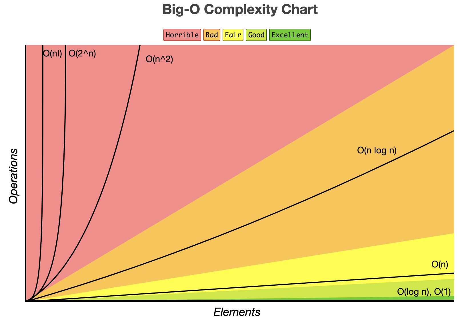
This is why an interview question isn't just about getting a correct answer; it's about finding a solution that lives in the green or yellow zones.

Key Takeaways

• Time Complexity measures how the runtime of an algorithm scales with the input size, not the exact time in seconds.
• Big-O Notation is the standard for expressing the worst-case time complexity.
• The Three Rules: Always analyze the worst case, and when simplifying, drop constants and drop non-dominant terms.
• Iterative Complexity: You can often determine complexity by analyzing loop structures:
  • No loops (or loops with a fixed number of iterations): $O(1)$
  • A single loop up to $n$: $O(n)$
  • A nested loop up to $n$: $O(n^2)$
  • A loop that halves the problem size at each step: $O(\log n)$
• Recursive Complexity: This is analyzed using a recurrence relation, which expresses the time of a problem in terms of its subproblems.

Next Steps

Well done on completing your first lesson! You've just learned the language that we'll use to evaluate every algorithm and data structure from now on.

In our next lesson, we will explore the other side of the coin: Space Complexity. You'll learn how to analyze the memory usage of an algorithm, including the often-hidden memory consumed by the recursion stack.