In our previous lesson, we explored the cause-specific hazard (CSH) model. We learned that it's an excellent tool for asking etiologic questions—questions about the direct effect of a covariate on the instantaneous rate of a specific event among those who are still event-free. However, we also discovered its crucial limitation: a higher cause-specific hazard does not necessarily mean a higher overall probability of that event occurring, because the covariate's effect on competing events complicates the picture.
This leaves an important question unanswered: how do we model a patient's overall prognosis? How do we estimate the effect of a covariate on the actual probability of an event happening over time, fully accounting for the fact that a competing event might happen first?
This lesson introduces the solution: the Fine-Gray subdistribution hazard model. By the end of our session, you will be able to interpret the results of this model and understand why it is the preferred tool for prognostic questions in the presence of competing risks.
A New Kind of Hazard: The Subdistribution Hazard
To address the challenge of predicting cumulative incidence directly, researchers R.J. Fine and J.H. Gray developed a model based on a different type of hazard function, called the subdistribution hazard (SDH). The genius of their approach lies in redefining the risk set—the group of individuals considered "at risk" of the event at any given time.
Recall that for the cause-specific hazard, the risk set at time includes only those who are currently event-free. If a person experiences a competing event, they are removed from the risk set.
The subdistribution hazard model does something radically different.
In a Fine-Gray model for Event 1, the risk set at time includes:
- All individuals who are still event-free.
- All individuals who have already experienced a competing event (e.g., Event 2).
This is a counter-intuitive idea. Why would we keep someone who died of a competing cause in the risk set for our event of interest? The video clip below introduces this concept.
Competing risks in survival analysis
This clip from the Population Data BC video introduces the subdistribution hazard function and explains its unique risk set.
Please watch from this section. Focus on the speaker's definition of the risk set and how it differs from the cause-specific hazard's risk set.
This unconventional definition can be difficult to grasp. Let's look at a visual representation to make it concrete. The image below contrasts the risk sets for the Cause-Specific Hazard (CSH) and Subdistribution Hazard (SDH) models over time.
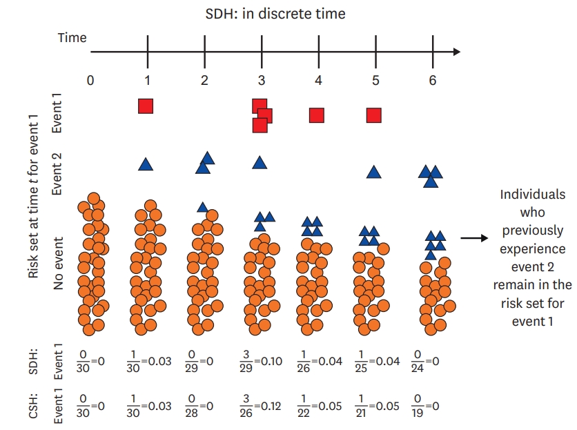
Look closely at the columns representing the "Risk set at time t for event 1". For the CSH calculation at the bottom, the denominator shrinks as individuals experience either Event 1 (red squares) or Event 2 (blue triangles). For the SDH calculation, the denominator only shrinks when individuals experience Event 1. As the note on the right says, "Individuals who previously experience event 2 remain in the risk set for event 1."
Why This Strange Risk Set Works
This strange risk set is a clever mathematical construction designed to achieve one specific goal: to create a hazard function that has a direct, one-to-one relationship with the Cumulative Incidence Function (CIF). Remember, the CIF is the true probability of an event occurring by a certain time in the presence of competing risks.
By keeping subjects who had competing events in the risk set, the model effectively "holds them accountable" and prevents the incidence of the event of interest from being artificially inflated. This direct link is why the Fine-Gray model is sometimes called a CIF regression model.
The following video segment and reading explain this crucial connection.
Competing risks in survival analysis
Here, the speaker explains why the counter-intuitive subdistribution hazard function is so useful: it is directly linked to the cumulative incidence function (CIF).
Watch from this segment. The key takeaway is that this hazard function was specifically chosen to allow researchers to make claims about the CIF.
Now, let's see this described in text. The following reading formally defines the subdistribution hazard and emphasizes its link to the CIF.
Practical recommendations for reporting Fine‐Gray model analyses ...
This article clarifies the interpretation of the Fine-Gray model. This section introduces the core concepts.
In the "INTRODUCTION" section, start reading from the paragraph that begins "In survival analysis". Focus on the formal definitions of the cause-specific hazard (formula 2) and the subdistribution hazard (formula 3), and note how the article explicitly states that the subdistribution hazard model allows one to estimate the effect of covariates on the CIF.
Interpreting the Subdistribution Hazard Ratio (sHR)
Because the Fine-Gray model directly models the CIF, the interpretation of its coefficients—the subdistribution hazard ratios (sHRs)—is different from the cause-specific hazard ratios (CS-HRs) we saw in the last lesson.
An sHR tells you about the effect of a covariate on the cumulative incidence of the event of interest. This is exactly what we need for prognostic questions.
The following video provides a clear set of rules for interpretation.
Competing risks in survival analysis
This clip gives a concise guide on how to interpret the output from a Fine-Gray model.
Please watch from this part. The speaker lists five key points for interpreting an sHR. Pay close attention to the final point about what the magnitude of the sHR does and does not mean.
Let's break down these crucial rules of interpretation:
-
Direction of Effect: The sHR tells you the direction of a covariate's effect on the cumulative incidence.
- An sHR > 1 implies that the covariate is associated with an increased cumulative incidence (a higher probability of the event occurring over time).
- An sHR < 1 implies that the covariate is associated with a decreased cumulative incidence (a lower probability).
- An sHR = 1 implies no association.
-
Magnitude of Effect (The Important Caveat): While the direction is clear, the magnitude is not. An sHR of 1.5 does not mean that the cumulative incidence is 1.5 times higher or that the probability increases by 50%. It simply means the incidence is higher. The further the sHR is from 1, the stronger the effect on the CIF, but the relationship is not a simple multiplicative one.
The following reading reinforces this distinction between interpreting the direction and the magnitude.
Practical recommendations for reporting Fine‐Gray model analyses ...
This is the most important section of this article for our purposes. It contrasts the interpretation of CSH models with Fine-Gray models.
In Section 2, "INTERPRETING REGRESSION COEFFICIENTS FROM COMPETING RISK REGRESSION MODELS," please read subsection 2.3. Subdistribution hazard model regression coefficients—effect on the CIF. Read the text from the beginning of the subsection. The author makes the point very clearly that a test of the sHR is a test for the effect on the CIF, but that you cannot infer that the magnitudes are the same.
Etiology vs. Prognosis: Choosing the Right Model
We have now covered two distinct regression models for competing risks. The choice between them depends entirely on your research question.
- For Etiologic Questions: If you want to understand the underlying biological mechanism or the direct effect of a covariate on the rate of an event, use the Cause-Specific Hazard Model. Its CS-HR is a rate ratio.
- For Prognostic Questions: If you want to predict a person's overall probability of experiencing an event or the effect of a covariate on absolute risk, use the Fine-Gray Subdistribution Hazard Model. Its sHR tells you the effect on the cumulative incidence.
This distinction is fundamental. The video below concludes with this exact advice, summarizing when to use each model.
Competing risks in survival analysis
This final summary from the video recaps the main recommendations for analyzing competing risks data, emphasizing the importance of matching the model to the research objective.
Watch the summary from this section. The speaker cites a key paper by Lau et al. that neatly frames the CSH model as being for "etiological questions" and the Fine-Gray model for "prognosis" and "absolute risk."
For a quick reference on these concepts, the following resource provides excellent summaries.
Fine–Gray Model (Subdistribution Hazard) - MetricGate
This webpage from MetricGate is a useful quick-reference guide.
Please review the short sections Key Concepts, Interpreting Results, and the answers to the first four questions in the Frequently Asked Questions section. These provide concise definitions and reinforce the key interpretation points.
Conclusion
In this lesson, we have added the second major tool for competing risks regression to our toolkit: the Fine-Gray subdistribution hazard model. Unlike the cause-specific model, which focuses on event rates, the Fine-Gray model is designed to answer questions about overall probability and prognosis.
Here are the key takeaways:
- The Fine-Gray model is used for prognostic questions about the cumulative incidence function (CIF), which represents the probability of an event occurring over time.
- It is based on the subdistribution hazard (SDH), which uses a unique risk set: individuals who experience a competing event remain "at risk" for the event of interest.
- This construction creates a direct link between the model's coefficients and the CIF.
- The subdistribution hazard ratio (sHR) from a Fine-Gray model indicates the direction of a covariate's effect on the cumulative incidence. An sHR > 1 means higher incidence; an sHR < 1 means lower incidence.
- Crucially, the magnitude of the sHR is not a direct measure of the change in probability (e.g., sHR of 2.0 does not mean a doubling of risk).
You are now equipped to distinguish between the two primary modeling approaches for competing risks and, most importantly, to correctly interpret the results of each based on the research question being asked.
This lesson concludes our exploration of competing risks. In our final lesson for this module, we will briefly touch on another common complexity in survival data: recurrent events, where individuals can experience the same type of event multiple times.