The previous lesson separated two router safeguards: load-balancing loss encourages a better spread of assignments, while z-loss constrains a property of the raw logits. Neither guarantees that every expert can process every assignment it receives in a particular batch.
This lesson puts a capacity on each expert. You will calculate the number of available slots and the assignments that exceed them, making the top- counting convention explicit. Allow about 40 minutes for the video excerpts, short readings, and worked examples.
From selected experts to available slots
A router may select an expert for a token even when that expert already has a full batch of work. Capacity-limited routing resolves this by giving each expert a fixed number of slots for the routing group. An assignment that cannot obtain a slot overflows. With top- routing, one token makes assignments, so it is important not to equate an overflowing assignment with an entirely dropped token.
Watch the setup and slot-allocation portions of this demonstration. You can skip its intervening router-logit walkthrough, which revisits earlier material.
MoE Token Routing Explained: How Mixture of Experts Works (with Code)
Watch “MoE Token Routing Explained: How Mixture of Experts Works (with Code)” from Hugging Face for a visual account of expert slots and overflow.
Start with expert slots: identify the four tokens, four experts, top-2 selections, and two slots per expert. Then watch slot allocation, focusing on how an expert's running assignment count identifies entries beyond its slots. When the narration calls a token “dropped,” inspect its individual expert selections: in top-2 routing, losing one contribution need not remove the other.
The Switch Transformer illustration shows the same resource constraint for top-1 routing. Its dotted line marks an assignment that cannot fit; its white expert slots show room reserved but unused.
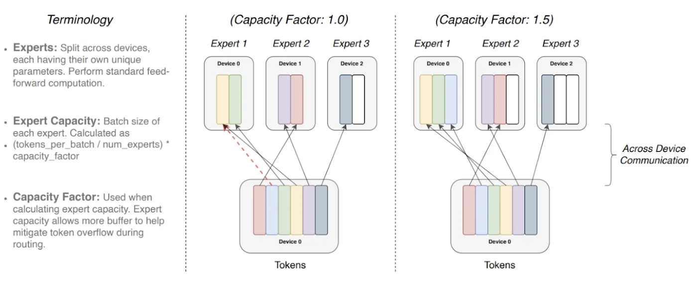
Read the figure caption and the accompanying capacity explanation in the paper. The paper uses top-1 routing, so we will extend its accounting to top- immediately afterward.
[PDF] Scaling to Trillion Parameter Models with Simple and Efficient Sparsity
Read Figure 3 and Section 2.2 of the Switch Transformer paper by Fedus, Zoph, and Shazeer to connect the buffer illustration to its capacity-factor formula.
On printed p. 5, read Figure 3's terminology and figure caption. Then, in Section 2.2, “Efficient Sparse Routing,” find “Distributed Switch Implementation.” Read the capacity explanation through the formula that follows it. Focus on what is being divided equally and what the capacity factor adds.
A capacity factor gives headroom, not a promise that routing will be balanced. Even when the average load fits, a popular expert can overflow while another has empty slots.
State the top- convention before calculating
Let be the number of input tokens in one routing group, the number of eligible experts, and the number of distinct experts selected per token. Before any capacity restriction, the router makes
token–expert assignments. The equal-share load is therefore assignments per expert, not necessarily .
For this lesson, we use capacity factor and the following integer-slot convention:
Here is the capacity of each expert within that routing group. The ceiling means that a fractional proposed capacity is rounded up to a usable whole slot. Other implementations can use different rounding or minimum-capacity rules; a calculation is reproducible only when those rules are stated. For top-1, , so this reduces to the equal-share expression shown in the Switch Transformer figure, with our ceiling rule added.
The Megatron-Core documentation explicitly includes top- in its capacity formula and distinguishes capacity-limited dropping from dropless dispatch. Read its short numbered list to compare conventions.
Mixture of Experts package — Megatron-LM - NVIDIA Documentation
Read the Megatron-Core documentation's three dispatch strategies to see why top-k multiplies the assignment budget and why capacity is optional in a dropless configuration.
Find the numbered list about dropping strategies immediately before the “Fine-tuning Mixtral Models” heading. Read all three strategies. In the second item, focus on the formula using tokens per rank, top-k, capacity factor, and number of experts. That is a per-rank accounting convention: do not compare a per-rank capacity with assignment counts pooled across a different routing group.
To interpret any capacity report, first fix its scope. In the example below, the routing group is one flattened batch of tokens, and both capacity and expert loads are measured for that same batch.
Count overflow from the actual assignments
Capacity can be calculated before the router makes its choices. Overflow cannot. Let be the number of assignments selecting expert , counted before any are rejected. These loads satisfy
If each expert keeps at most assignments, its overflow count and retained count are
The total number of overflowing assignments is . Which particular assignments lose their slots requires a priority or ordering policy; how many overflow at each expert does not.
Consider six tokens, three experts, and top-2 routing. Suppose the selections are:
| Token | Selected experts |
|---|---|
| 0 | 0, 1 |
| 1 | 0, 1 |
| 2 | 0, 2 |
| 3 | 0, 1 |
| 4 | 0, 2 |
| 5 | 1, 2 |
There are assignments. Counting appearances gives expert loads , which sum to 12 as they must. With , the per-expert capacity is
Expert 0 has five requests for four slots, so its overflow is one. Experts 1 and 2 have zero overflow. One of twelve assignments overflows, despite capacity equaling the average load. If assignments are admitted in token order, token 4's selection of expert 0 is the one that overflows; its selection of expert 2 still fits. The exact survivor would change under a different admission policy, but the overflow count remains one.
Changing only shows what the buffer buys:
| Capacity factor | Slots per expert | Overflow by expert | Total overflow |
|---|---|---|---|
| 0.75 | 3 | 3 | |
| 1.0 | 4 | 1 | |
| 1.5 | 6 | 0 |
At , the three experts have only nine slots in total for twelve assignments: at least three must overflow regardless of how evenly routing is distributed. At , there are twelve slots in total, yet one assignment still overflows because the slots are partitioned by expert. At , this batch fits, but some reserved slots go unused.
Checks that prevent misleading capacity calculations
Two quick checks catch many mistakes. First, verify that the measured loads sum to , not , for top- routing. Second, compare loads with the integer capacity , not with the fractional quantity inside the ceiling.
Rounding can matter even for top-1. For , , , and , our rule gives . Loads of produce one overflowing assignment. Rounding down instead would give two slots per expert—and only six slots for seven assignments—so it describes a different policy with a different answer.
The total number of slots, , offers a useful lower bound:
If there are fewer slots than assignments, some overflow is unavoidable. The reverse is not true: enough slots overall do not prevent an individual expert from filling up. Nor does capacity itself redirect an overflowing assignment to an idle expert; a fallback would be an additional routing policy.
Finally, report the right unit. For top-2, “three dropped assignments” does not tell you whether three tokens each lost one expert contribution or whether some tokens lost both. Expert loads alone determine , but not the number of tokens left with no expert contribution.
Takeaways
Calculate capacity from the number of assignments, , divided among experts and multiplied by the stated capacity factor. Under this lesson's rounding convention, each expert has slots. Then count its pre-capacity selections : precisely of its assignments overflow. Always keep the routing group, rounding rule, and distinction between assignments and tokens explicit.
The next lesson will turn those counts into capacity-limited dispatch, specifying which overflowing contributions to omit while preserving the transformer's residual path.