A capacity limit changes more than the shape of an expert’s input buffer: when routing is uneven, it changes which expert contributions reach the model. Earlier in this module, capacity was defined per expert and overflow was handled by dropping expert contributions while leaving the transformer’s residual path intact.
This lesson holds a skewed set of routing decisions fixed and compares two ways of executing it. You will track dropped assignments and peak expert batch size, then use those counts to interpret the padding and workload trade-offs. Plan on about 40 minutes, including the short video, reading, and worked audit.
Two ways to handle uneven expert loads
First, watch a visual account of capacity overflow and the alternative to fixed-size expert batches.
Mixture of Experts (MoE), Visually Explained
Watch “Mixture of Experts (MoE), Visually Explained” by Jia-Bin Huang for its visual comparison of fixed-capacity and dropless expert computation.
Watch capacity overflow for the fixed-size buffer, dropped-token, and residual-path explanation. Continue with dropless computation; focus on why unequal expert batch sizes need not imply dropping or padding every expert to the same size.
The crucial distinction is between a routing decision and an executed assignment. With top- routing, each token requests experts. A capacity-limited dispatcher accepts at most assignments for each expert; an overflow assignment contributes no expert output under the dropping policy used here. A dropless dispatcher executes every requested assignment, so its expert batch sizes follow the router’s actual, potentially unequal counts.
Read the two implementation descriptions below for the shape constraint behind that choice. Stop after the dropless section’s unpermute + combine bullet; the later discussion of multi-device buffers is beyond this lesson’s comparison.
Dropless MoE Training in JAX with Primus-Turbo — ROCm Blogs
Read the capacity-factor and dropless-routing sections of this ROCm Blogs article to connect fixed buffers, overflow, padding, and variable-length expert groups.
In “dense_matmul: Capacity-Factor Dropping,” read from the paragraph beginning “The simplest way to make MoE shapes static” through the end of that section, fixed-capacity routing. Focus on the formula containing the number of tokens, top-k, and number of experts. Then, in “sparse_matmul: Dropless Routing,” start with the paragraph explaining that dropless routing. Continue through the “unpermute + combine” bullet, where expert results return to token order. Focus on the unequal group sizes, not the subsequent multi-device implementation details.
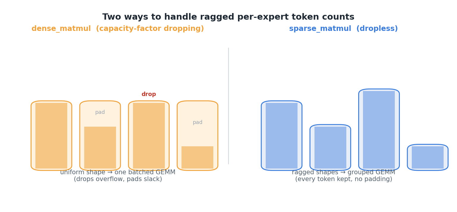
The image shows why “no drops” is not the same as “raise the capacity until nothing drops.” Both can preserve every assignment on a particular batch, but the raised-capacity version still reserves the same number of slots for every expert.
Fix the routes, then count what changes
Consider eight tokens, four experts, and top- routing. Each row gives a token’s selected experts in slot order. These choices stay identical in every comparison; only the dispatch policy changes.
| Token | Selected experts |
|---|---|
| each | |
| each | |
There are requested assignments. Before imposing capacity, the expert counts are . The mean is four assignments per expert, but expert 0 has seven. That difference between mean load and peak load drives the comparison.
For this lesson, use the explicit convention
where tokens, selected experts, experts, and is the capacity factor. Thus the capacity is . When an expert has more than requests, keep them in ascending token order and drop the rest. Do not reroute overflow or renormalize the surviving gates; either change would define a different policy.
At , capacity is four. Expert 0 accepts through and drops its assignments from . Expert 1 accepts through and drops its assignment from . Experts 2 and 3 accept all their requests. That is four dropped assignments, not four discarded tokens: each affected token retains its other selected expert in this particular batch.
Here is the complete comparison. “Peak executed” is the largest actual per-expert batch; “reserved slots” counts fixed buffer positions, including padding.
| Dispatch policy | Capacity | Dropped assignments | Executed counts by expert | Peak executed | Reserved slots | Padding slots |
|---|---|---|---|---|---|---|
| Capacity factor | 4 | 4 | 4 | 16 | 4 | |
| Capacity factor | 6 | 1 | 6 | 24 | 9 | |
| Capacity factor | 8 | 0 | 7 | 32 | 16 | |
| Dropless | No fixed cap | 0 | 7 | No fixed buffers | 0 |
The numbers reveal two different meanings of “peak.” At capacity factor , the uncapped demand still peaks at seven, but only four assignments reach the busiest expert. At capacity factor , actual work peaks at seven even though each expert has an eight-slot buffer. Dropless routing also executes a batch of seven at expert 0, without allocating equal eight-slot expert buffers under this simple accounting.
For fixed buffers, padding is reserved slots minus accepted assignments. At factor , for example, slots hold accepted assignments, leaving nine padding slots. These are shape and slot counts, not measured FLOPs or step times: a particular kernel may avoid some arithmetic on padding, and a dropless kernel has its own handling costs. The counts alone do not establish which implementation is faster.
Audit the comparison independently of expert weights
A small routing audit makes the accounting reproducible before introducing expert computation. It uses the same token-order priority as the worked example and records which selected-expert slots survive:
routes = (
    (0, 1), (0, 1), (0, 1), (0, 1),
    (0, 2), (0, 2), (0, 3), (1, 2),
)

def audit(routes, num_experts, capacity=None):
    requested = [0] * num_experts
    executed = [0] * num_experts
    dropped = [0] * num_experts
    surviving_slots = [[] for _ in routes]

    for token, choices in enumerate(routes):
        for slot, expert in enumerate(choices):
            requested[expert] += 1
            if capacity is None or executed[expert] < capacity:
                executed[expert] += 1
                surviving_slots[token].append(slot)
            else:
                dropped[expert] += 1

    return requested, executed, dropped, surviving_slots

for capacity in (4, 6, 8, None):
    requested, executed, dropped, slots = audit(routes, 4, capacity)
    padding = 0 if capacity is None else 4 * capacity - sum(executed)
    print(capacity, requested, executed, sum(dropped),
          max(executed), padding)
The four output rows reproduce the table’s requested counts, executed counts, drops, peak executed batch, and padding. In the capacity-four run, surviving_slots also shows that every token still has one selected-expert contribution. That is a property of these routes, not a guarantee of top- capacity-limited routing: both assignments for a token could overflow on another batch. If none survives, the dropped expert branch supplies no output for that token under this policy, while the transformer’s residual path still carries its representation.
This audit deliberately omits gate values and expert networks. Their inclusion would not change the assignment counts. In a full layer, the combine step uses the surviving selected-expert slots to place weighted outputs back at their original token positions.
What the two metrics tell you—and what they do not
Dropped assignments measure lost expert contributions. On this fixed batch, increasing capacity from four to six reduces drops from four to one; dropless dispatch reduces them to zero. Capacity eight also produces zero drops here, but reserves 32 slots for 16 real assignments. A different, more skewed batch could require a different capacity to avoid overflow.
Peak expert batch size measures concentrated work. Dropless dispatch exposes the router’s seven-assignment peak directly. Capacity four caps executed work at four by discarding three requests to that expert; it does not make the underlying routing balanced. Capacity eight preserves the seven-assignment peak while presenting uniform eight-slot buffers. This is why utilization reports should distinguish pre-capacity requests from executed counts.
Neither metric alone determines model quality or throughput. Dropped contributions can affect training, but the loss change requires training or evaluation evidence. Likewise, unequal dropless groups may create a busy-expert bottleneck, while fixed buffers may spend storage—and potentially computation—on padding. The MegaBlocks paper reports a quality cost from token dropping in its experiments, but its measured trade-off should not be treated as a performance prediction for this eight-token example.
Key takeaways
For the same routing demand, capacity factor drops four of 16 assignments and limits the peak executed expert batch to four. Dropless routing drops none and executes the full peak of seven. Raising capacity can remove drops on this batch, but uniform buffers then contain substantial padding. Always report whether an “expert count” means requests before capacity, contributions actually executed, or allocated buffer slots.
The next module moves from this fixed-batch accounting to short training runs, where validation loss and held-out routing patterns can show whether the observed expert usage is useful specialization rather than merely a skewed count.