Welcome back. Last lesson, you calculated router logits and applied softmax to obtain a probability for every expert. For the example token, experts through had logits , and all four received nonzero probabilities. This lesson adds the decision that makes the layer sparse: selecting only the top experts. You will then compare two ways to weight their outputs—keeping their original full-softmax probabilities or renormalizing those probabilities over the selected experts. Allow about 35–40 minutes, including the video and numerical walkthrough.
Selecting experts is a separate decision
Softmax preserves the ordering of logits: the expert with the highest logit also has the highest probability. Top- selection takes the indices of the highest values for each token. If for our four-expert example, the selected indices are and . Experts and do not run for this token, even though their full-softmax probabilities are positive.
The distinction is between a preference distribution and a compute decision. The router can score every expert cheaply, but the expensive feed-forward computation is performed only by the selected experts. With distinct scores, either the logits or the full-softmax probabilities give the same top- indices.
MoE Token Routing Explained: How Mixture of Experts Works (with Code)
Watch “MoE Token Routing Explained: How Mixture of Experts Works (with Code)” from Hugging Face for a visual account of selection and sparse gate weights.
Watch top-k selection to see how the router’s logit matrix yields expert indices for each token. Continue through sparse normalization, focusing on why unselected experts receive zero weight when softmax is applied after masking their logits. Stop before the discussion of expert slots and capacity.
Selecting indices does not yet settle how strongly to weight the two expert outputs. That depends on which set of experts the gate weights are normalized over.
Full-softmax weights versus selected-expert weights
Recall the full-softmax probabilities from the previous lesson:
| Expert | Logit | Full-softmax probability | Selected for top-2? |
|---|---|---|---|
| Yes | |||
| Yes | |||
| No | |||
| No |
The full-softmax probabilities sum to across all four experts. If we keep the original probabilities for experts and and set the others to zero, the surviving weights sum to only . Masking has removed probability mass; it has not redistributed it.
One valid gate convention uses those surviving values unchanged:
Another convention renormalizes over the selected set :
For , dividing by the selected mass gives approximately and . These two weights sum to . Expert still outweighs expert ; renormalization changes the scale, not their ranking or their relative weight.
The following charts show the same distinction with a different token and eight experts. There, experts and are selected, rather than experts and as in our numerical example.
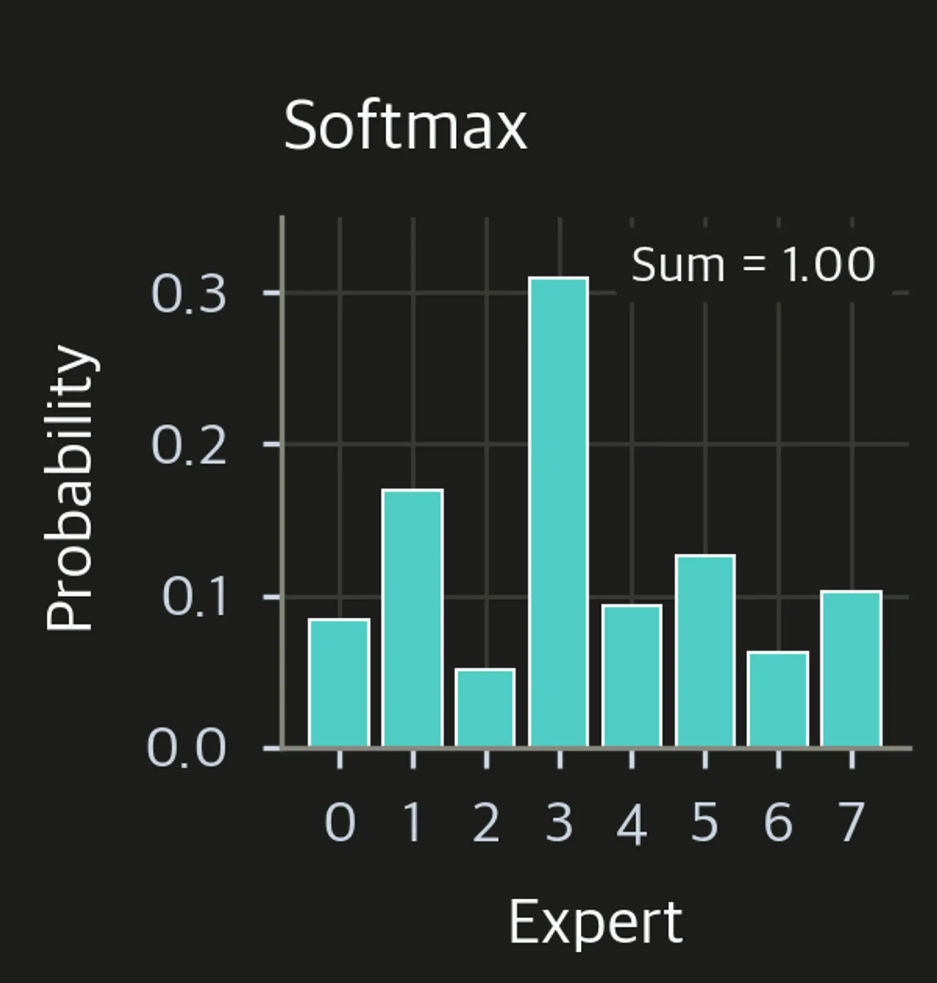
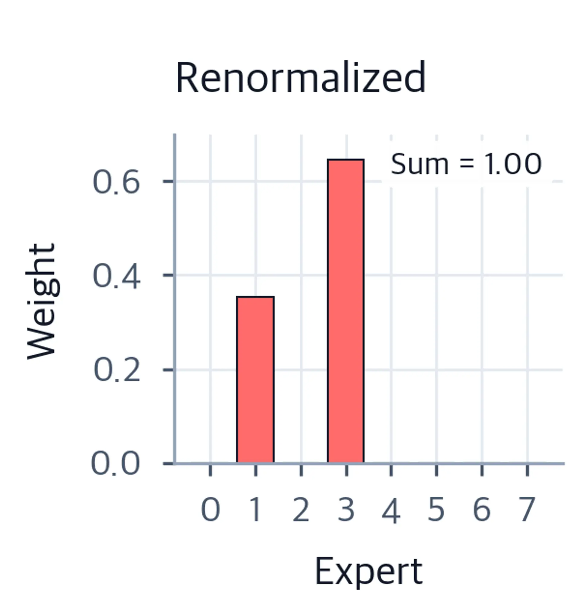
Why might the distinction matter? If is expert ’s output for token representation , the MoE sublayer combines the selected outputs as
For the same selected experts and expert outputs, using full-softmax gates produces an MoE output equal to times the output produced by renormalized gates in our example. That does not make full-softmax gating inherently an error: the conventions define different output scales, and implementations may deliberately choose either one. The key is to know which convention a model uses. The transformer’s residual connection is separate; this comparison concerns the MoE contribution, not the entire block output.
Two equivalent ways to renormalize
You do not have to compute a full softmax and then divide selected probabilities to obtain renormalized gates. Because every full-softmax probability has the same denominator, that denominator cancels:
Thus, softmax over only the selected logits gives the same renormalized weights. In our example, applying softmax to logits gives approximately . Equivalently, one can replace unselected logits with negative infinity and apply softmax across all expert positions; those positions then receive zero weight.
Here is a compact PyTorch check using the logits already calculated. The returned indices and weights occupy corresponding top- slots:
import torch

logits = torch.tensor([[2.0, 1.0, 0.0, -1.0]])  # one token, four experts

selected_logits, indices = logits.topk(k=2, dim=-1)
probs = logits.softmax(dim=-1)

full_gates = probs.gather(dim=-1, index=indices)
renorm_gates = selected_logits.softmax(dim=-1)

print(indices)        # [[0, 1]]
print(full_gates)     # approximately [[0.6439, 0.2369]]
print(renorm_gates)   # approximately [[0.7311, 0.2689]]
full_gates is a pair of values taken from a four-expert distribution. renorm_gates is a distribution over the two selected experts. In a larger token batch, these operations act along the last dimension, so every token gets its own indices and weights.
Two boundary cases sharpen the distinction. If equals the total number of experts, nothing is excluded and the two gate conventions coincide. If , renormalizing over the sole selected expert gives it weight , whereas keeping its full-softmax probability generally gives it a weight below . A later lesson will examine why that top-1 difference also matters for gradients; for now, it is enough to keep selection and weighting conceptually separate.
Takeaway
Top- routing chooses which experts execute for each token; gate weights determine how their outputs are combined. Full-softmax gates retain the selected experts’ probabilities from a distribution over all experts, so their sum may be below one. Renormalized gates divide by the selected probability mass—or, equivalently, apply softmax to the selected logits—so the executed experts’ weights sum to one.
Next, you will use the fact that only experts execute per token to distinguish a model’s total parameters from its per-token active parameters.