Welcome back. In the previous lesson, you separated the discrete choice of expert indices from the differentiable weights on selected expert outputs. Now the question is more concrete: when those operations appear in PyTorch, which axis represents tokens, experts, or a token’s selected-expert slot? This lesson traces those axes through a small router-and-expert scaffold. It uses renormalized top-2 gates, with no capacity limit or routing noise, so the indexing is visible before those complications are added.
From a token batch to routing indices
Watch the implementation portion of Hugging Face’s MoE Token Routing Explained: How Mixture of Experts Works (with Code). Concentrate on the shapes and on the two indices returned when the code finds tokens assigned to an expert; you do not need its later capacity machinery for this lesson.
MoE Token Routing Explained: How Mixture of Experts Works (with Code)
Hugging Face’s “MoE Token Routing Explained: How Mixture of Experts Works (with Code)” provides a visual-to-code bridge for the router and expert bank.
Watch the components for the feed-forward expert, router, and collection of experts. Then watch routing shapes: notice the flattened token batch, router logits, top-k indices, and renormalized weights. Finish with dispatch and return, focusing on why torch.where returns two indices and why index_add_ adds rather than replaces output rows.
The picture below shows the same routing problem as queues: each token appears in the queues of its two selected experts. An expert’s queue can contain several tokens, while another expert’s queue can be empty. The picture uses eight experts; the smaller code example below uses four.
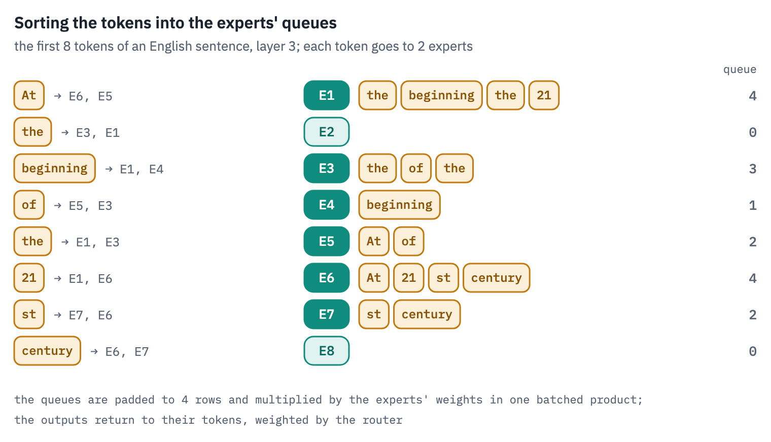
There are two different notions of “slot” worth separating immediately. A token’s selected-expert slot is its position among its top- choices: slot 0 for its highest-ranked choice, slot 1 for its second choice. A position within an expert’s queue is something else. The scaffold below needs the former to retrieve the correct gate weight; it does not allocate fixed queue positions.
A minimal PyTorch scaffold
Let the input have shape : batch size, tokens per sequence, and hidden width. Set , the number of token representations. There are experts, each with an intermediate width , and the router selects experts per token. The scaffold uses ModuleList so that each expert has independent feed-forward weights.
import torch
from torch import nn
from torch.nn import functional as F


class SparseExpertLayer(nn.Module):
    def __init__(self, d, h, n_experts, k):
        super().__init__()
        assert 1 <= k <= n_experts
        self.k = k
        self.router = nn.Linear(d, n_experts, bias=False)
        self.experts = nn.ModuleList([
            nn.Sequential(
                nn.Linear(d, h),
                nn.GELU(),
                nn.Linear(h, d),
            )
            for _ in range(n_experts)
        ])

    def forward(self, x):
        B, C, D = x.shape
        tokens = x.reshape(B * C, D)                 # [T, D]

        logits = self.router(tokens)                 # [T, N]
        probs = F.softmax(logits, dim=-1)            # [T, N]
        top_probs, expert_idx = probs.topk(
            self.k, dim=-1
        )                                            # both [T, k]
        gate = top_probs / top_probs.sum(
            dim=-1, keepdim=True
        )                                            # [T, k]

        out = torch.zeros_like(tokens)               # [T, D]
        for expert_id, expert in enumerate(self.experts):
            token_idx, choice_slot = torch.where(
                expert_idx == expert_id
            )                                        # both [M]

            if token_idx.numel() == 0:
                continue

            expert_in = tokens[token_idx]            # [M, D]
            expert_out = expert(expert_in)            # [M, D]
            weight = gate[token_idx, choice_slot]
            weight = weight.unsqueeze(-1)            # [M, 1]
            out.index_add_(
                0, token_idx, weight * expert_out
            )

        return out.reshape(B, C, D)                   # [B, C, D]
Read the forward pass as a sequence of shape contracts. reshape(B * C, D) combines only the batch and sequence axes. For a token originally at batch position and sequence position , its flattened row is . The hidden vector remains intact; the router and every expert still receive features per token. The final reshape restores the transformer-compatible shape.
The router’s linear layer maps each vector to logits, so row of logits contains one score per expert for token . Softmax acts along the last axis, independently for each token. topk then returns two tensors: floating-point top_probs and integer expert_idx. Their entries must be read together: top_probs[t, s] belongs to expert expert_idx[t, s].
The division creates renormalized selected gates. Although probs[t] sums to one across all experts, its selected entries generally do not. gate[t] sums to one across the selected entries. This is the gate convention whose gradient behavior you traced in the previous lesson.
Follow the paired indices through one expert
Use , , , , , and . Then tokens is , logits is , and both expert_idx and gate are . Suppose their values for one forward pass are:
token row t       0       1       2       3
expert_idx[t]   [2, 0]  [1, 2]  [2, 3]  [0, 1]
gate[t]         [.7,.3] [.8,.2] [.6,.4] [.9,.1]
Consider the loop iteration for expert 2. The comparison expert_idx == 2 produces a Boolean matrix of shape . torch.where returns the coordinates of its True entries as paired, one-dimensional index tensors:
token_idx   = [0, 1, 2]
choice_slot = [0, 1, 0]
Thus expert 2 receives token rows 0, 1, and 2. It is token 1’s second choice, so its weight for that token is gate[1, 1], not gate[1, 0]. Paired advanced indexing, gate[token_idx, choice_slot], yields [.7, .2, .6] with shape . Indexing tokens[token_idx] yields ; expert 2 maps those three vectors through widths , , and , returning .
unsqueeze(-1) changes the weights to . Multiplication broadcasts each weight across its corresponding output features. Finally, index_add_(0, token_idx, ...) adds those three weighted rows into rows 0, 1, and 2 of out.
Why add? Expert 0 will also produce a contribution for token 0, while expert 3 will produce one for token 2. Those later contributions belong in the same output rows as earlier ones. After all expert iterations, each row contains the sum of that token’s selected expert outputs, weighted by its gates. The output is not in expert-queue order: token_idx directs every contribution back to its original flattened token row.
The loop also handles an expert with no selected tokens. In that iteration token_idx has length zero, and continue avoids calling its feed-forward network on an empty batch. Here , the number of rows processed in an iteration, can differ for every expert. It is not , and it is not necessarily .
Two ways to store the same expert bank
The scaffold’s ModuleList makes the index trace easy to see: expert_id identifies one independently parameterized network, and tokens[token_idx] forms its variable-length input batch. For comparison, read the “Expert Layers” portion of nanoMoE: Mixture-of-Experts (MoE) LLMs from Scratch. It shows expert weights stored together and applied with batched matrix multiplication instead of a Python loop over expert modules.
nanoMoE: Mixture-of-Experts (MoE) LLMs from Scratch in ...
Read Cameron Wolfe’s “Expert Layers” section to compare the scaffold’s ModuleList with a bank of expert-weight tensors.
Under “Expert Layers,” begin with the paragraph explaining how the ordinary feed-forward component is replaced. Read through the implementation explanation. Then inspect the MLPExperts code block immediately below it, from class MLPExperts through its final return x. Focus on the first dimension of c_fc and c_proj, and on what shape x must have for torch.bmm to work. Stop before “Creating an MoE.”
In that grouped layout, a first-layer weight bank has shape , and a second-layer bank has shape . If the input batches are arranged as , torch.bmm can produce for the first projection and for the second. Here represents a common batch length in that tensor layout; our loop instead lets each expert process its own rows. These are different storage and batching choices for the same per-token routing relationship. Neither changes the need to remember which original token and which selected-expert slot each expert computation belongs to.
The useful invariant is:
The scaffold realizes this expression by gathering tokens expert by expert, then accumulating their contributions token by token. The indices determine where computation happens and where its result returns; the gate determines how much that result contributes.
Conclusion
A reliable shape trace starts with , flattens to , obtains routing scores , and retains paired expert indices and gates . Within an expert iteration, torch.where pairs each original token row with its selected-expert slot. That pair retrieves both the input vector and the correct gate; index_add_ returns weighted outputs to the original token rows without overwriting other expert contributions.
The next lesson takes the router portion of this scaffold and implements its top- indices and gate weights directly.