Last lesson showed why a balancing number can change when you regroup the same tokens into different microbatches. Now you will hold the batch definition fixed and change one routing hyperparameter: the expert capacity factor. The aim is to run two short training runs and judge them using validation loss, expert utilization, dropped assignments, and step time together. A lower drop rate alone is not a complete result.
This lesson uses a small, reproducible top-1 MoE experiment. It is deliberately modest: it tests your measurement and comparison procedure, not which capacity factor is best for a large model.
What the ablation changes
With tokens in each dispatch batch, experts, and top-1 routing, this experiment sets each expert’s capacity to
where is the capacity factor. Each token requests one expert. If more than tokens request an expert, only its first assignments in flattened batch order are processed; the others receive no expert contribution. The transformer’s residual path still carries their representations forward.
We will compare with . The model architecture, initial weights, token batches, optimizer, training steps, top-, and auxiliary-loss coefficient remain the same. Capacity is the only configured difference. Once training begins, the two models can learn different routes; identical initial weights do not imply identical routing throughout the runs.
Switch Transformers: Scaling to Trillion Parameter Models with Simple and Efficient Sparsity
Read the Switch Transformer paper’s capacity definition and its capacity-factor comparison. They motivate both the drop measurement and the need to report quality alongside speed.
In Section 2.2, “Efficient Sparse Routing,” find the subsection “Distributed Switch Implementation.” Read the capacity discussion. Focus on why spare capacity reduces overflow but can have a cost. Then go to Section 2.3, “Putting It All Together: The Switch Transformer”: read Table 1 and its context, ending with the speed caveat immediately after the table. Compare rows within a model family rather than treating every row as an otherwise identical capacity-factor run. The paper’s displayed capacity formula is for its Switch, top-1 setting; the experiment below also uses top-1.
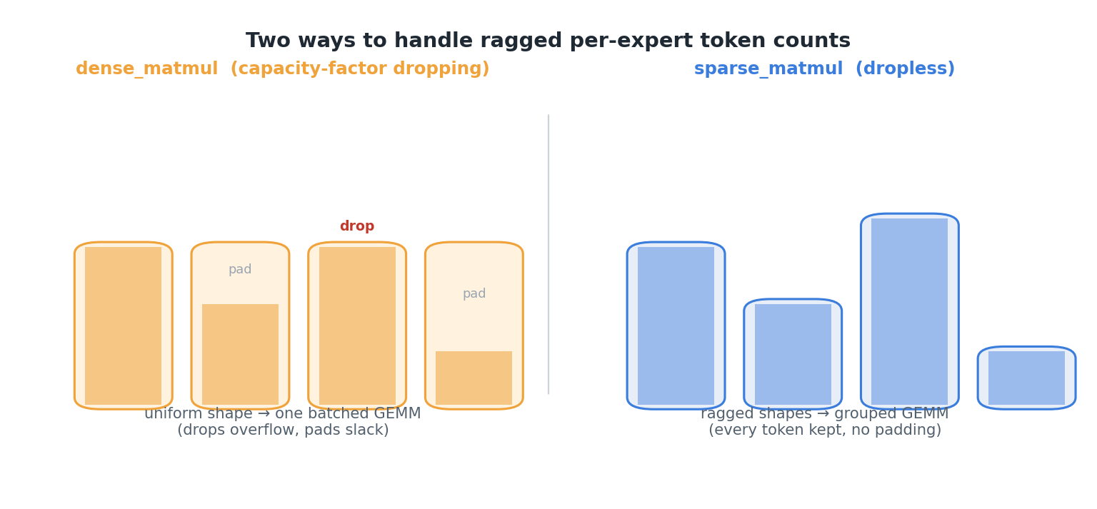
A capacity factor also has an implementation-dependent timing effect. A fixed-shape implementation may pad unused expert slots; a ragged implementation may instead process only assignments that exist. The following diagram distinguishes those mechanisms, not the measured performance of the code you are about to run.
Run a paired experiment
The script is self-contained so that you can run the ablation even if your earlier tiny transformer uses different class names. Its synthetic next-token sequences have two identifiable token groups. It uses a causal attention layer and replaces its feed-forward contribution with four top-1 experts. The full-softmax probability of the selected expert weights its output; it is not a renormalized top-1 gate. The load-balancing coefficient is fixed at in both runs, and validation loss excludes that auxiliary term.
import math
import statistics
import time

import torch
from torch import nn
from torch.nn import functional as F

torch.manual_seed(23)
device = torch.device("cuda" if torch.cuda.is_available() else "cpu")
if device.type == "cpu":
    torch.set_num_threads(1)

V, D, E = 16, 32, 4
B, S = 16, 12
STEPS, WARMUP = 80, 10

def make_batches(n, seed):
    g = torch.Generator().manual_seed(seed)
    batches = []
    offsets = torch.arange(S).view(1, S)
    for _ in range(n):
        group = torch.randint(0, 2, (B, 1), generator=g)
        start = torch.randint(0, 8, (B, 1), generator=g)
        x = group * 8 + (start + offsets) % 8
        y = group * 8 + (start + offsets + 1) % 8
        batches.append((x.to(device), y.to(device)))
    return batches

train_batches = make_batches(STEPS, seed=101)
val_batches = make_batches(8, seed=202)

class TinyMoE(nn.Module):
    def __init__(self, capacity_factor):
        super().__init__()
        self.capacity_factor = capacity_factor
        self.embed = nn.Embedding(V, D)
        self.attn = nn.MultiheadAttention(D, 2, batch_first=True)
        self.norm_attn = nn.LayerNorm(D)
        self.norm_expert = nn.LayerNorm(D)
        self.router = nn.Linear(D, E)
        self.experts = nn.ModuleList([
            nn.Sequential(nn.Linear(D, 64), nn.ReLU(), nn.Linear(64, D))
            for _ in range(E)
        ])
        self.head = nn.Linear(D, V)

    def forward(self, x):
        batch_size, seq_len = x.shape
        h = self.embed(x)
        causal_mask = torch.ones(
            seq_len, seq_len, device=x.device, dtype=torch.bool
        ).triu(1)
        u = self.norm_attn(h)
        attn_out, _ = self.attn(
            u, u, u, attn_mask=causal_mask, need_weights=False
        )
        h = h + attn_out

        flat = self.norm_expert(h).reshape(-1, D)
        prob = self.router(flat).softmax(dim=-1)
        chosen = prob.argmax(dim=-1)
        intended = torch.bincount(chosen, minlength=E)
        capacity = math.ceil(
            self.capacity_factor * flat.shape[0] / E
        )

        expert_out = torch.zeros_like(flat)
        kept = []
        for expert_id, expert in enumerate(self.experts):
            rows = torch.nonzero(
                chosen == expert_id, as_tuple=True
            )[0][:capacity]
            kept.append(rows.numel())
            if rows.numel():
                contribution = expert(flat.index_select(0, rows))
                contribution = (
                    contribution * prob[rows, expert_id].unsqueeze(-1)
                )
                expert_out = expert_out.index_add(
                    0, rows, contribution
                )

        h = h + expert_out.reshape(batch_size, seq_len, D)
        fraction = intended.float().detach() / flat.shape[0]
        mean_prob = prob.mean(dim=0)
        balance_loss = E * (fraction * mean_prob).sum()
        return (
            self.head(h),
            intended.detach(),
            torch.tensor(kept, device=x.device),
            balance_loss,
        )

def synchronize():
    if device.type == "cuda":
        torch.cuda.synchronize()

# Capture one initialization; each run loads its own copy.
torch.manual_seed(303)
initial = {
    key: value.clone()
    for key, value in TinyMoE(1.0).state_dict().items()
}

def run(capacity_factor):
    model = TinyMoE(capacity_factor).to(device)
    model.load_state_dict(initial)
    optimizer = torch.optim.AdamW(model.parameters(), lr=3e-3)
    step_times = []
    train_intended = torch.zeros(E, dtype=torch.long, device=device)
    train_kept = torch.zeros_like(train_intended)

    model.train()
    for step, (x, y) in enumerate(train_batches):
        synchronize()
        start = time.perf_counter()

        optimizer.zero_grad(set_to_none=True)
        logits, intended, kept, balance_loss = model(x)
        cross_entropy = F.cross_entropy(
            logits.reshape(-1, V), y.reshape(-1)
        )
        loss = cross_entropy + 0.01 * balance_loss
        loss.backward()
        optimizer.step()

        synchronize()
        elapsed = time.perf_counter() - start
        if step >= WARMUP:
            step_times.append(elapsed)
        train_intended += intended
        train_kept += kept

    model.eval()
    val_loss_sum = 0.0
    val_tokens = 0
    val_intended = torch.zeros_like(train_intended)
    val_kept = torch.zeros_like(train_intended)
    peak_intended = 0

    with torch.no_grad():
        for x, y in val_batches:
            logits, intended, kept, _ = model(x)
            val_loss_sum += F.cross_entropy(
                logits.reshape(-1, V), y.reshape(-1),
                reduction="sum"
            ).item()
            val_tokens += y.numel()
            val_intended += intended
            val_kept += kept
            peak_intended = max(
                peak_intended, int(intended.max().item())
            )

    def counts(tensor):
        return tensor.cpu().tolist()

    return {
        "cf": capacity_factor,
        "val_ce": val_loss_sum / val_tokens,
        "train_dropped": int(
            (train_intended - train_kept).sum().item()
        ),
        "val_dropped": int(
            (val_intended - val_kept).sum().item()
        ),
        "val_assignments": int(val_intended.sum().item()),
        "intended_by_expert": counts(val_intended),
        "kept_by_expert": counts(val_kept),
        "peak_batch_expert": peak_intended,
        "median_step_ms": 1000 * statistics.median(step_times),
        "p90_step_ms": 1000 * sorted(step_times)[
            int(0.9 * (len(step_times) - 1))
        ],
    }

for cf in (1.0, 2.0):
    result = run(cf)
    print(result)
Budget approximately 15–20 minutes to inspect, run, and, if needed, adapt this code to your earlier model. Its validation set is generated separately from the training stream, but the task is intentionally simple. Do not interpret a small difference in its loss as evidence that one capacity factor will generalize better elsewhere.
The accounting has two distinct populations. intended_by_expert counts choices before capacity; kept_by_expert counts expert contributions actually computed. For this top-1 script,
Here a dropped assignment also means a token missed its sole expert contribution. That equivalence would not generally hold for top-2 routing, where one contribution could be dropped while the other survives. The script’s capacity applies per dispatch batch, not over all 80 training steps or all validation batches.
Read the result without conflating its causes
Put the two printed dictionaries side by side. A compact report should include validation cross-entropy, intended and kept counts for each expert, training and validation drop rates, peak intended expert load in a validation batch, and median and 90th-percentile training step time. Divide a drop count by its corresponding intended-assignment count before comparing runs; raw totals are useful here because the runs have equal batch counts, but rates make the convention explicit.
First check the mechanical effect. With the same routes on a given batch, a higher capacity cannot increase that batch’s overflow. After training, however, routes need not remain the same. Therefore a changed validation drop count combines more room per expert with any routing changes learned during training. Intended counts reveal the latter; kept counts reveal the work actually executed. If one expert receives most intended assignments, a low drop rate at does not establish healthy utilization.
Next examine quality. Validation cross-entropy is the primary task measure; the auxiliary balance loss is a training term, not part of the reported validation score. If the larger capacity reduces drops without a clear validation improvement, possible explanations include an already small drop rate, insufficient training, or variation in this tiny experiment. Avoid assigning a cause from two final numbers alone. For a more reliable follow-up, repeat the same two configurations with several paired initialization and data seeds, keeping each seed’s two runs matched.
Finally examine time. The script times forward, backward, and optimizer work for each training step, synchronizing around GPU measurements and excluding ten initial steps from its summaries. It does not measure data generation, validation, expert-parallel communication, or a padded fixed-shape kernel. In this particular Python-loop implementation, increasing capacity can change how many expert rows are evaluated; it need not have the same speed effect as changing capacity in the paper’s implementation. A faster step with more drops is not automatically a better system, nor is a slower step with lower validation loss automatically a worse one. State the quality–drop–time trade-off you observed under this implementation.
One further control matters: this script retains the first assignments to an overloaded expert in flattened batch order. That makes overflow reproducible but can favor earlier positions. If you replace that policy with randomized retention, keep the policy and its random seeds identical across both capacity settings, and report the change as a new experiment rather than merging its results into this pair.
Takeaway
A controlled routing ablation changes one configured hyperparameter while keeping the model initialization, data, training schedule, and measurement scope fixed. For capacity factor, report intended utilization, executed utilization, dropped assignments, validation loss, and step time: each answers a different question. Your two runs provide an interpretable small-system comparison, not a universal capacity recommendation.
The final lesson will use this kind of evidence alongside correctness, numerical stability, memory, and communication checks to decide whether the implementation is ready to scale.