Hello. Last lesson established that a sparse layer can return plausible tensors even when dispatch or combination is wrong. Those correctness checks matter before performance profiling: a fast expert-parallel run is not useful if its tokens reached the wrong experts.
This lesson focuses on a different failure: one rank holds up an otherwise correct training step. You will learn to read per-rank assignment counts alongside dispatch, expert-compute, and return timings, then distinguish an overloaded expert owner from slow communication or misleading wait time. This is a diagnosis lesson, not an invitation to tune the router before finding the bottleneck.
What a rank is waiting for
In expert parallelism, each rank owns a subset of experts. A token may be routed to an expert on another rank. The dispatch exchange delivers its hidden state to that owner; after expert computation, a return exchange sends the result back for weighted combination. The diagram shows the basic all-to-all pattern: each rank contributes data to several destinations and receives the pieces addressed to it.
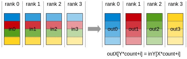
The unit to count is an expert assignment, not necessarily a distinct token. With top- routing, one token can contribute assignments, possibly to experts on different ranks. For a dropless batch of tokens, the sum of the expert owners’ received assignment counts is . If capacity limits drop contributions, count assignments after that policy when relating counts to actual expert work.
Read the short expert-parallelism portion of the lecture slides before examining a timing trace. It provides the workflow and the reason the busiest rank can set the pace.
Lecture 5: Parallelism Strategies - Scaling Transformers ...
These Scalable AI lecture slides connect MoE routing to all-to-all communication and rank imbalance. Read the indicated slides rather than the full lecture.
On slide 29 / 107, under “MoE workflow: router → dispatch → experts → combine,” follow the four operations. On slide 30 / 107, “Visualizing AllToAll,” use the chunk description to interpret the diagram. Then read slide 32 / 107, “Load balancing: the ‘slowest expert’ sets step time,” from the imbalance warning. On slide 34 / 107, “EP group sizing and placement,” focus on what to profile. You can skip the intervening capacity-factor and inference slides for this lesson.
A useful first distinction is between where work lands and where time is reported. The rank with the most assignments may spend longest in expert computation. Another rank may report the longest return call because it finished computing early and entered the return exchange first. A long call can contain waiting for a peer; it need not mean that peer’s network link is slow.
Read counts and timings as one timeline
Consider two ranks, each owning experts of the same size. This simplified forward trace uses dropless routing. Both ranks enter dispatch together; expert computation begins once dispatch finishes; a rank enters the return exchange when its local experts finish. The reported return duration includes time spent waiting within that exchange.
| Measurement | Rank 0 | Rank 1 |
|---|---|---|
| Received expert assignments | 160 | 40 |
| Dispatch interval | 0–5 ms | 0–5 ms |
| Expert-compute interval | 5–21 ms | 5–9 ms |
| Return interval | 21–25 ms | 9–25 ms |
| Reported return duration | 4 ms | 16 ms |
Both ranks finish the layer at 25 ms. Rank 0 is the compute straggler, despite rank 1’s much larger reported return duration. Rank 1 reaches the return exchange at 9 ms, twelve milliseconds before rank 0 reaches it. In this illustrative trace, its 16 ms return duration consists of roughly 12 ms awaiting the late peer and 4 ms completing the exchange. The intervals—not just the duration column—reveal the direction of the wait.
The assignment counts strengthen that interpretation. Rank 0 receives four times as many assignments, and its 16 ms expert-compute interval is four times rank 1’s 4 ms interval. That proportionality is unusually neat; real grouped expert kernels have launch overhead, variable efficiency, and different per-expert batch shapes. Still, the counts and the location of the extra time agree.
An average-to-maximum count ratio gives a quick measure of rank-level skew. Here the mean is 100 assignments and the maximum is 160, so the ratio is . It is a load proxy, not a prediction that GPU utilization or throughput is exactly 62.5%. The trace itself shows the relevant consequence: rank 1 finishes its expert work early but cannot finish the layer independently.
The most common timing mistake would be to read the final row alone and announce “rank 1 has a return-communication problem.” The corrective habit is to record when each rank enters and leaves each phase. If a profiler offers only per-phase durations, inspect adjacent phases and synchronize their timelines before attributing a long collective call to the network.
When the counts do not explain the delay
Unequal counts are evidence of unequal workload, but they do not explain every slow step. Suppose both ranks receive 100 assignments and show similar expert-compute intervals, yet dispatch and return each take much longer than on a comparable batch. There is no count-based case for an overloaded expert owner. Investigate communication: how many assignments actually cross ranks, which links they use, message sizes, and the dispatch and combine kernels.
For tokens with top- selection, hidden width , and bytes per activation element, let be the fraction of assignments whose experts live on another rank. Ignoring metadata and protocol overhead, the cross-rank activation payload is approximately
One copy travels to the expert owner and one result travels back. This estimate helps explain why equal received counts can coexist with different communication behavior: a batch can route mostly to local experts or mostly to remote ones. It does not predict latency by itself. Collectives also pay for coordination, and their implementation and hardware topology matter.
A practical case study illustrates two different causes that a slow MoE run might conceal. Read the communication-kernel investigation and the separate investigation of an extreme rank-count imbalance. Do not assume either cause applies to your trace without matching evidence.
Field Notes on Scaling MoE Expert Parallelism with DeepEP | Nous Research
These Nous Research field notes show how profiled communication kernels and destination-rank counts led to different diagnoses. Concentrate on the evidence used, not on copying the implementation-specific fixes.
In “November 14 - Scaling Expert Parallelism Linearly,” find “Problem 1: Intranode kernels scale poorly with expert parallelism.” Read from the profiler investigation; skim the kernel tables for the relative dispatch and combine costs. Separately, in “November 25 - Fixing Gradient Norm Explosion in MoE Training,” read from the routing investigation. Notice how destination-rank counts prompted a check of router scores and weights. Stop there; the later zero-token grouped-GEMM issue concerns a different failure.
The second investigation offers an important caution. A rank receiving nearly all assignments might reflect data-dependent routing, but an extreme, persistent concentration can also indicate a router or implementation fault. In the field notes, zero router scores led top- selection to choose experts placed on the same rank. Counts identified the symptom; inspecting scores and weights established the cause. Do not prescribe a load-balancing change solely from the count histogram.
There is also a middle case: rank totals look balanced, but one rank computes longer. Inspect counts per expert, not only their sums per rank. One rank might have a very large batch for one expert while another has several smaller expert batches; grouped-kernel efficiency and expert implementation can make their compute times differ. If both rank and per-expert counts are comparable, profile the expert kernels and check for other work sharing the device before blaming routing.
A disciplined diagnostic record
For each profiled step, preserve enough information to reconstruct both the workload and the critical path:
- Routing and placement: Count assignments received by every expert and sum them by owner rank. Record dropped assignments separately if capacity limits are enabled. Keep the expert-to-rank mapping with the trace.
- Traffic: Count assignments sent from each source rank to each destination rank. A destination histogram describes expert load; a source–destination matrix also shows remote traffic.
- Phase boundaries: Record entry and completion times for dispatch, expert computation, and return on every rank—not just each phase’s duration. Include any local packing or combination time consistently.
- Timing method: Distinguish CPU time spent launching or waiting for operations from elapsed GPU work. For asynchronous GPU operations, use appropriate device events and synchronization when collecting a completed trace. Compare ranks from the same step and align their timelines.
- Repeatability: Compare several representative steps. A one-batch routing spike and a persistent placement or communication problem call for different responses.
Read that record in order. First verify that assignment totals match the routing and capacity policy; the previous lesson’s identity tests guard against counting a wrongly dispatched workload. Next, identify the late rank before return and ask whether its received counts and expert-compute time rise together. Finally, inspect the exchanges. If a short-compute rank has a long return interval because it entered early, its return time is largely a consequence of the straggler. If counts and compute are balanced but exchange intervals dominate, communication deserves investigation.
This reasoning is more reliable than adding one rank’s reported phase durations and comparing the largest entries. Distributed operations can overlap, and collective calls can include waiting. The quantity to explain is the step’s critical path: which rank and phase delayed completion for everyone else?
Key takeaways
An expert-parallel straggler is diagnosed by combining assignment counts with a synchronized phase timeline. High received counts together with late expert-compute completion point toward an overloaded owner; a peer’s long return call may simply record its wait. Balanced counts and compute shift attention toward dispatch, return, placement, or kernel overhead. Per-expert counts and source–destination traffic prevent rank totals from hiding important differences.
The next lesson uses skewed dropless counts to estimate activation memory. The same assignment histogram that exposes a compute straggler can also reveal a rank at risk of exceeding its memory budget.