Applying Gradient Boosting Models

1. The Gradient Boosting Workflow with XGBoost

XGBoost, which stands for "eXtreme Gradient Boosting," is an optimized, scalable, and highly performant implementation of the gradient boosting algorithm. While the theory you learned applies, libraries like XGBoost include many engineering enhancements to make them fast and effective.

We'll follow a step-by-step coding tutorial from StatQuest. The example task is to predict customer churn—a classic binary classification problem.

Step 1: Data Preparation

As with any modeling task, the first step is preparing the data. This involves not just loading and cleaning, but also formatting the data in a way the algorithm can understand. Two key steps for tree-based models are handling categorical features and missing data.

• One-Hot Encoding: Gradient boosting models, like decision trees, require numerical inputs. Categorical features like payment_method (e.g., 'Mailed Check', 'Credit Card') must be converted into a numerical format. One-hot encoding is a standard technique that creates new binary (0/1) columns for each category. This prevents the model from incorrectly assuming an ordinal relationship between categories (e.g., that 'Credit Card' is somehow "greater than" 'Mailed Check').
• Handling Missing Data: A unique feature of XGBoost is its built-in capability to handle missing values. The standard approach, as you'll see in the video, is to identify them and then let XGBoost's default mechanism decide how to treat them during the tree-building process. When combined with one-hot encoding, this is handled very efficiently using sparse matrices, meaning the zeros (representing non-applicable categories or missing values) don't take up memory.

This first video segment walks through these critical data preparation steps.

Step 2: Build and Evaluate a Preliminary Model

Once the data is prepared, we can build our first XGBoost model. The process involves:

1. Splitting Data: Separate features (X) from the target (y). Then, split into training and testing sets. For classification with an imbalanced target variable (like customer churn, where fewer people churn than stay), it's crucial to use stratification. This ensures that the proportion of the minority class is the same in both the training and test sets, leading to a more reliable evaluation.
2. Initial Training: We'll use the scikit-learn compatible XGBClassifier. A key practical tool here is early stopping. Instead of guessing the number of trees to build, we can tell XGBoost to monitor performance on a validation set and stop training if the performance doesn't improve for a specified number of rounds. This prevents overfitting and finds a reasonable number of trees automatically.
3. Initial Evaluation: We'll use a confusion matrix to see how well our first model performs.

This next segment covers these steps and reveals a common problem with imbalanced datasets.

As you saw, the initial model is great at identifying customers who don't churn, but terrible at identifying those who do. This is because the model can achieve high accuracy by simply predicting the majority class all the time. Our next step is to fix this.

Step 3: Optimizing for Imbalanced Data

To improve our model's ability to detect the minority class, we need to tell it that misclassifying a "churner" is a more serious error than misclassifying a "non-churner". XGBoost provides a hyperparameter specifically for this purpose: scale_pos_weight.

The recommended value for scale_pos_weight is the ratio of the number of negative class samples to positive class samples. For example, if we have 1000 non-churners (negative class, 0) and 100 churners (positive class, 1), the ratio would be 1000/100 = 10. By setting scale_pos_weight=10, we are telling the model to weight the errors on the positive class ten times more heavily. This forces the model to work harder at correctly identifying churners.

While other parameters (max_depth, learning_rate) can also be tuned (often with cross-validation), scale_pos_weight is the most direct tool for tackling class imbalance.

2. A Faster Alternative: LightGBM

XGBoost is incredibly powerful, but for very large datasets, training time can become a factor. LightGBM is another gradient boosting framework from Microsoft that is designed to be highly efficient and is often significantly faster than XGBoost.

The main reason for its speed is a different tree-building strategy.

• XGBoost uses level-wise growth. It splits all the nodes at the current depth before moving to the next level, creating balanced trees.
• LightGBM uses leaf-wise growth. It identifies the single leaf that will yield the largest reduction in loss and splits only that one. This results in asymmetric trees but converges on the solution much more quickly.

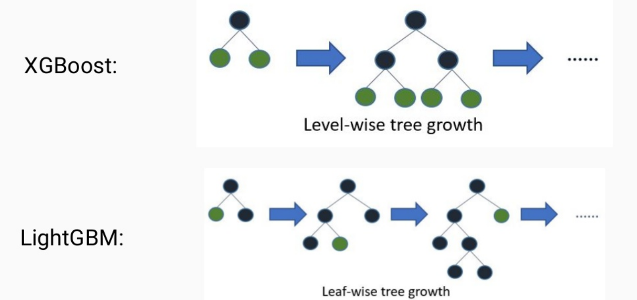
In practice, applying LightGBM is very similar to XGBoost, as it also has a scikit-learn compatible API (LGBMClassifier). The core workflow of data prep, training, and tuning remains the same.

# A simple example of applying LightGBM
import lightgbm as lgb
from sklearn.model_selection import train_test_split
from sklearn.metrics import accuracy_score

# Assume X_encoded and y are your preprocessed data from the XGBoost steps
X_train, X_test, y_train, y_test = train_test_split(X_encoded, y, test_size=0.2, random_state=42, stratify=y)

# Instantiate the classifier
# LightGBM also has a parameter for imbalanced data, 'is_unbalance=True' or using 'scale_pos_weight'
lgbm = lgb.LGBMClassifier(objective='binary',
                          is_unbalance=True, # A simple way to handle imbalance
                          random_state=42)

# Train the model
lgbm.fit(X_train, y_train)

# Make predictions and evaluate
y_pred = lgbm.predict(X_test)
print(f"LightGBM Accuracy: {accuracy_score(y_test, y_pred):.2f}")

For a more detailed walkthrough of applying LightGBM, including parameter tuning, the Kaggle notebook LightGBM Classifier in Python (ID: LINK) is an excellent resource you can explore on your own.

Conclusion

In this lesson, you have walked through the practical application of gradient boosting models, from raw data to an optimized, evaluated classifier.

Key Takeaways:

• Applying XGBoost involves a workflow of data preparation (one-hot encoding), data splitting (using stratification for imbalance), training (using early stopping), and evaluation.
• For imbalanced classification problems, the scale_pos_weight hyperparameter is a critical tool for forcing the model to pay more attention to the minority class.
• Optimizing for the minority class often involves a trade-off: you improve recall for that class at the expense of precision for the majority class. This is often a desirable trade-off from a business perspective.
• LightGBM is a faster alternative to XGBoost, primarily due to its leaf-wise tree growth strategy, compared to XGBoost's level-wise approach.

Preview of the Next Lesson:
You have now applied both Random Forests (a bagging method) and Gradient Boosting models. But when should you choose one over the other? In our next lesson, we will directly compare the strengths and weaknesses of Random Forests and Gradient Boosting, discussing their performance, tuning complexity, and suitability for different types of problems. This will equip you with the strategic knowledge to select the best ensemble method for your task.