Random Forests: Enhancing Robustness through Feature Randomness

1. From Bagging to Random Forests

A Random Forest is an extension of the bagging method we just learned. It uses the same core principles of bootstrapping and aggregation, but with one crucial addition: feature randomness.

Let's see a step-by-step guide to building a Random Forest. This process introduces a second layer of randomness on top of the bootstrapping we saw in the last lesson.

To recap the video's key steps:

1. Bootstrap the Data: Just like in bagging, create a new dataset by sampling rows with replacement from the original training data.
2. Build a Decision Tree with a Twist:
   • Start building a normal decision tree.
   • However, at each node, before you look for the best split, randomly select a subset of the available features.
   • Find the best split only among that random subset of features.
   • Continue this process down the tree.
3. Repeat: Repeat steps 1 and 2 many times (hundreds is common) to create a "forest" of diverse trees.
4. Aggregate Predictions: To make a prediction for a new data point, let all the trees in the forest vote (for classification) or average their predictions (for regression).

This second layer of randomness is the defining characteristic of a Random Forest.

2. Why Feature Randomness Creates Robust Models

In the previous lesson, we noted that bagged trees can be correlated. If one feature is a very strong predictor, most of the bootstrapped trees will probably use that feature for their first split. This makes the trees structurally similar and limits the amount of variance reduction we get from averaging them.

Random Forests directly combat this problem. By forcing each split to consider only a random subset of features, it prevents individual trees from all latching onto the same dominant predictor.

To understand why this diversity is so powerful, let's explore the concept of tree correlation.

The main takeaway is that by making the trees less correlated, we get a greater reduction in variance when we average their predictions.

Some trees will be built without seeing the strongest predictor at all, forcing them to discover other, more subtle patterns in the data. While these individual trees might be weaker, their errors are different from the errors of the other trees. When we average them all together, these diverse errors cancel each other out more effectively, leading to a more robust and accurate final model.

This video provides another clear explanation of this exact point.

In summary, the robustness of a Random Forest comes from this two-pronged approach to creating diversity:

• Bagging ensures trees are trained on different data samples.
• Feature randomness ensures trees are built using different sets of predictors.

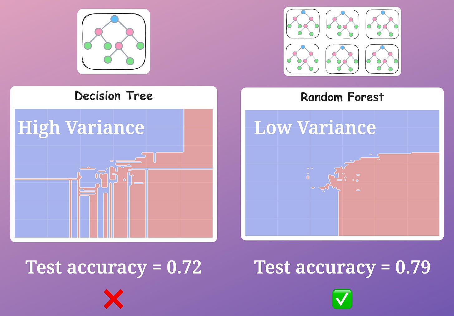
The result is a model that is much less sensitive to the specific noise in the training data, as seen by the smoother decision boundary and higher accuracy in the image below.

3. Applying Random Forests: Key Hyperparameters

Now that you understand the "why," let's touch on the "how." When you apply a Random Forest in practice (for example, using Python's scikit-learn library), there are two main hyperparameters that control the randomness we've discussed.

The two most important hyperparameters for controlling the model's structure are:

1. n_estimators: This is the number of trees in the forest. It's the same idea as in bagging. More trees are generally better (up to a point of diminishing returns), but they increase the computational cost. A common starting point is 100 or more.

2. max_features: This is the size of the random subset of features to consider at each split. This is the key hyperparameter that makes a Random Forest different from a standard bagged ensemble.

   • Effect: A smaller max_features increases randomness and de-correlates the trees, which reduces variance but can slightly increase the bias of individual trees (since they might not get to see the best predictors). A larger max_features makes the trees more similar and the model behaves more like standard bagging.
   • Common Settings: For a dataset with m total features, common defaults are max_features = sqrt(m) for classification and max_features = m/3 for regression. These are good starting points, but this hyperparameter is often a prime candidate for tuning to get the best performance.

Conclusion

You've now progressed from single decision trees to bagging, and finally to Random Forests. You can now explain not just how a Random Forest is built, but also articulate why its specific design—particularly the use of feature randomness—makes it one of the most robust and widely used algorithms in machine learning.

Key Takeaways:

• A Random Forest is an ensemble of decision trees that improves on bagging by adding feature randomness.
• At each split in a tree, only a random subset of features (max_features) is considered.
• This additional randomness de-correlates the trees, preventing them from all relying on the same few strong predictors.
• By averaging the predictions of these diverse, de-correlated trees, a Random Forest achieves a greater reduction in variance, leading to a more robust and accurate model.

Preview of the Next Lesson:
Random Forests and Bagging are known as parallel ensemble methods, where many independent models are built and their results are combined. In the next lesson, we will explore a fundamentally different approach to ensembles called Boosting. We will learn about Gradient Boosting, a sequential method where each new model is built to correct the errors of the previous one. This powerful technique focuses on reducing bias rather than variance.