Hello! Welcome to the final lesson of our first module on mathematical foundations.
In our last lesson, we demystified backpropagation, the powerful algorithm that calculates the gradient of a loss function. We saw how this gradient tells our model which "direction" to adjust its parameters to reduce error. Today, we'll explore the landscape that our model navigates using that gradient.
This brings us to today's learning outcome: to distinguish between convex and non-convex functions and explain the implications for optimization. Understanding this distinction is fundamental to grasping why some machine learning models are easy to train and guaranteed to find the best solution, while others, like deep neural networks, are much trickier and require a host of specialized techniques.
The Shape of the Problem: Convex vs. Non-Convex Landscapes
Imagine training a model is like being a hiker in a thick fog, trying to find the lowest point in a landscape. The gradient is your compass, always pointing downhill.
- If you're in a simple, bowl-shaped valley, following the "downhill" direction will inevitably lead you to the bottom. This is a convex landscape.
- But what if you're in a vast mountain range with countless valleys, pits, and flat plateaus? Your compass might lead you to the bottom of a small, high-altitude valley, while the deepest point in the entire range is miles away. This is a non-convex landscape.
Let's build a clear visual intuition for these two types of functions.
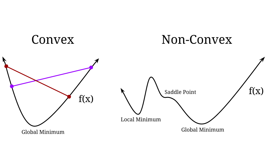
In machine learning, the "landscape" is the loss function, and its "location" is defined by the model's parameters. Our goal is to find the parameter values that correspond to the lowest point on this surface.

What Makes a Function Convex?
Let's formalize the visual intuition. A function is convex if a straight line drawn between any two points on its graph never goes below the graph itself.
To see this simple graphical test in action, watch the following video segment.
Difference between convex & non-convex cost function; what happens when cost function is non-convex?
The video 'Difference between convex & non-convex cost function' by CampusX provides a very clear, intuitive graphical definition.
Watch from 03:29 to 05:25. Focus on the simple 'line segment test' used to visually determine if a function is convex or not.
The most important property of a convex function for optimization is:
Any local minimum is also the global minimum.
This is a powerful guarantee. It means that if our gradient descent algorithm finds a point where the gradient is zero (a flat spot), we know we have found the single best possible solution.
Why is this true? Since you have some calculus background, we can look at a slightly more formal reason that is very intuitive. A convex function always lies above any of its tangent lines (or tangent hyperplanes in higher dimensions).
Convexity and The Principle of Duality
The video 'Convexity and The Principle of Duality' by Visually Explained offers a beautiful explanation for this key property.
Watch from 06:07 to 07:54. The core idea is that if a function is always above its tangent plane, and you find a point where the tangent plane is flat (i.e., the gradient is zero), that point must be the global minimum.
This property is why convex optimization problems are considered "solved." We have reliable methods that are guaranteed to work.
The Challenge of Non-Convexity
Non-convex functions are simply all functions that are not convex. Their graphs can have multiple dips and peaks, which creates significant challenges for optimization.
The primary challenge is the existence of local minima: valleys that are not the deepest point in the landscape. An optimization algorithm like gradient descent can easily get trapped in one of these, thinking it has found the solution when a much better one exists elsewhere.
Let's return to the CampusX video to see the implications of this.
Difference between convex & non-convex cost function; what happens when cost function is non-convex?
This segment clearly explains why non-convex functions are problematic for our optimization goal.
Watch from 06:17 to 08:37. Notice the distinction made between a 'local minima' and a 'global minima' and why an optimization algorithm might converge to the wrong one.
Test your understanding!
Imagine you are training two different machine learning models.
- Model A's loss function is convex.
- Model B's loss function is non-convex.
You train each model five times, each time starting with different random initial parameter values. What would you expect to observe about the final performance of the models from these five runs?
Show answer
- For Model A, you would expect all five training runs to converge to the exact same set of final parameters and achieve the same, optimal performance. Because the loss function is convex, there is only one minimum, and the optimizer will find it regardless of where it starts.
- For Model B, you would likely see different results from the five runs. Some runs might find a good local minimum and perform well, while others might get stuck in a poor local minimum and perform badly. The final performance is sensitive to the initial starting point.
Convexity in Practice: From Linear Regression to Neural Networks
So, how does this apply to the machine learning models you want to build? The distinction between convex and non-convex loss functions is one of the most important practical dividers in machine learning.
The following article provides a fantastic overview. It uses the "bowl" vs. "egg crate" analogy and directly connects these ideas to the models you will be using.
Convex vs Non-Convex Optimization
This article from TensorTonic, 'Convex vs Non-Convex Optimization', is a great summary of the practical implications of convexity in ML.
Please read the following three parts of the article: Start with the Introduction (from the top down to just before 'Convex Sets'). It sets the scene perfectly with the 'bowl' vs 'egg crate' analogy. Then, read the section titled 'The Convex World: Where Life is Good'. It lists common ML models with convex loss functions. Finally, read the section 'The Non-Convex Reality: Deep Learning's Jungle'. It explains why neural networks are non-convex and the hazards this creates.
To summarize the key points:
-
Convex Models (The "Good" World):
- Linear Regression (with Mean Squared Error loss)
- Logistic Regression (with Cross-Entropy loss)
- Support Vector Machines (SVMs)
- Implication: For these models, you are guaranteed to find the globally optimal parameters. They are reliable, predictable, and their results are reproducible.
-
Non-Convex Models (The "Jungle"):
- Neural Networks / Deep Learning Models
- Decision Trees and many Ensemble models
- Implication: Training is not guaranteed to find the best solution. The process is sensitive to initialization and requires careful tuning and specialized optimization algorithms.
Why Does Deep Learning Work At All?
This raises a crucial question: if the loss landscapes of neural networks are such a complex, non-convex "jungle," why are they so incredibly effective? This was a major mystery for a long time, but researchers have uncovered some key insights.
Briefly, it turns out that in the very high-dimensional spaces where neural networks operate:
- Bad local minima are rare. Most local minima have a loss value that is very close to the global minimum's loss. So, getting stuck is often "good enough."
- Saddle points are more common than minima. These are points that are a minimum in some directions but a maximum in others (like the middle of a Pringles chip). While they can slow down training, modern optimizers are designed to escape them.
- The noise from using mini-batches of data (which we'll cover in the next module) helps "shake" the optimizer out of shallow valleys.
You can read more about this in the "Why Deep Learning Works Anyway" section of the TensorTonic article (LINK) if you are curious.
Conclusion
You have now reached the end of the first module and have built a solid mathematical foundation. Today's lesson was crucial for bridging theory and practice, explaining the why behind many of the challenges and choices in model training.
Key Takeaways:
- Convex functions are "bowl-shaped." They have a single global minimum, making optimization straightforward and reliable. Any local minimum is the global minimum.
- Non-convex functions have complex, "mountainous" landscapes with multiple local minima and saddle points. Optimization algorithms can get stuck in suboptimal solutions.
- This distinction explains why models like Linear and Logistic Regression are guaranteed to find an optimal solution, while training neural networks is an experimental process that is sensitive to factors like initialization and optimizer choice.
- Despite being non-convex, deep learning is effective because the properties of high-dimensional spaces make finding a "good enough" solution very likely.
Next Steps:
This lesson perfectly sets the stage for our next module, Optimization for Machine Learning. We will officially kick off our journey into how models are trained by first looking closely at loss functions. Then, we will dive deep into the mechanics of gradient descent, the algorithm we've been referencing, and learn how to implement and tune it to navigate both convex and non-convex landscapes effectively.