Residual Connections in Deep Networks

1. The Problem with Very Deep Networks

In the early days of deep learning, there was a race to build deeper models. However, researchers quickly ran into two major obstacles: the vanishing gradient problem and a surprising phenomenon known as the degradation problem.

The Vanishing Gradient Problem

We've touched on this before. During backpropagation, the gradients are calculated using the chain rule, which involves multiplying many small numbers together as the error signal travels backward from the output layer to the input layer. In a very deep network, this can cause the gradient to shrink exponentially, becoming so small that the weights of the early layers barely update. As a result, the initial layers of the network fail to learn effectively.

To understand this more formally, it's helpful to review the mechanics of backpropagation.

The Degradation Problem

Even more puzzling is the degradation problem. One might expect that a deeper model should, at worst, perform as well as a shallower one. After all, the deeper model could theoretically just learn to copy the behavior of the shallower model in its initial layers and treat the extra layers as identity functions (i.e., they just pass the input through unchanged).

In practice, this doesn't happen. Experiments showed that as "plain" networks (simple stacks of layers) got deeper, their accuracy on both the training and testing sets would first saturate and then quickly degrade.

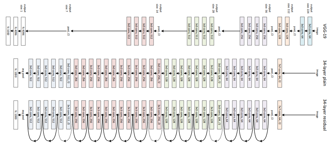
Why is learning an identity function so hard for a stack of non-linear layers? This is the central challenge that ResNet was designed to solve.

The following video provides an excellent visual summary of these problems.

2. The Solution: Learning the Residual

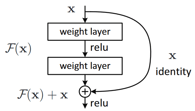
The insight behind Residual Networks (ResNets) is brilliantly simple. Instead of forcing a set of layers to learn a target mapping H(x), let's reframe the problem. We'll have the layers learn a residual function F(x) = H(x) - x.

The original mapping can then be calculated as:

This is implemented using a "shortcut" or "skip connection" that passes the input x directly to the end of the block and adds it to the output of the layers, F(x).

Why is this easier?
Imagine the ideal mapping is simply the identity function (H(x) = x).

• In a plain network, the stack of layers would have to learn to approximate the identity function, which is difficult.
• In a residual network, the layers just need to learn a residual F(x) that is equal to zero. It's much easier for a network to push its weights towards zero than to fine-tune them to approximate an identity mapping.

This reframing makes the network's job significantly simpler, especially when the optimal transformation is close to the identity.

3. The Residual Block in Detail

A residual block is the fundamental building block of a ResNet. A common variant consists of:

1. A 3x3 Convolutional Layer
2. A Batch Normalization Layer
3. A ReLU Activation Function
4. Another 3x3 Convolutional Layer
5. Another Batch Normalization Layer
6. An addition operation, where the input to the block (x) is added to the output of the second batch norm layer.
7. A final ReLU Activation Function.

The key is the "skip connection" in step 6. Let's look at this structure more closely.

4. How Residual Connections Enable Deeper Networks

Now we can connect the pieces and understand exactly how this architecture solves our two main problems.

Solving the Vanishing Gradient Problem

The skip connection creates an alternative path for the gradient to flow during backpropagation. The gradient can now flow backward through the identity connection uninterrupted. Since the derivative of the identity function (x) with respect to x is 1, the gradient is passed back directly, without being diminished by multiplications in the weight layers.

This acts like an express lane for the gradient, ensuring that even the earliest layers in a very deep network receive a strong error signal and can continue to learn effectively.

Solving the Degradation Problem

By making it easy to learn the identity function, residual blocks ensure that adding more layers can't hurt performance. In the worst-case scenario, the network can simply learn to set the weights of the extra layers to zero, making them identity mappings. The deeper model then becomes equivalent to the shallower model. This property, where deeper function classes contain the shallower ones, is called nested function classes. This guarantees that a deeper model will have a training error that is at least as low as its shallower counterpart.

5. A Practical Detail: Handling Dimension Mismatches

There's one final detail we need to address. What happens if the convolutional layers inside the residual block change the dimensions of the data? For example, a convolution with stride=2 will halve the height and width of the feature maps. In this case, we can't directly add the input x to the output F(x) because their shapes don't match.

There are two common solutions:

1. Zero-Padding: Pad the input x with zeros to match the new channel dimension. This is simple but adds no new learnable information.
2. 1x1 Convolution: Use a 1x1 convolutional layer on the skip connection itself. This is a very powerful technique. A 1x1 convolution can be configured with a specific stride and number of filters to intelligently downsample x and change its channel depth to precisely match the dimensions of F(x). This is the approach used in the original ResNet paper.

Conclusion

In this lesson, we explored a fundamental breakthrough in deep learning. We saw how simply stacking layers in "plain" networks leads to performance degradation and training difficulties due to vanishing gradients.

Key Takeaways:

• The Problem: Very deep networks are hard to train due to the vanishing gradient and degradation problems.
• The Core Idea: ResNets reframe the learning problem. Instead of learning a direct mapping H(x), the network learns a residual mapping F(x) = H(x) - x.
• The Mechanism: This is achieved via skip connections, which add the block's input x to its output F(x).
• The Benefit (Gradient Flow): Skip connections create an express lane for gradients to flow backward through the network, mitigating the vanishing gradient problem.
• The Benefit (Identity Mapping): Residual blocks can easily learn identity functions, solving the degradation problem and enabling the effective training of networks with hundreds or even thousands of layers.

This simple but powerful idea of the residual connection has been incredibly influential and is now a standard component not only in modern CNNs but also in other advanced architectures like Transformers, which we will see later in the course.

Preview of the Next Lesson:

So far, we have focused on architectures for processing static, spatial data like images. But what about sequential data, where order matters, such as time series or text? In our next lesson, we will pivot to a new class of models designed for this purpose, starting with the foundational architecture: the Recurrent Neural Network (RNN).