Hello! Welcome to your next lesson in our "Advanced Neural Network Architectures" module.
In our last session, we dove into the core of Convolutional Neural Networks (CNNs): the convolutional layer. We saw how it uses local connectivity and shared weights to efficiently extract features from spatial data like images, creating outputs called feature maps.
A key challenge, however, is that these feature maps can still be very large and sensitive to the exact position of features. If an object in an image shifts by just a few pixels, the feature map will also shift. Today, we'll tackle this exact problem by exploring pooling layers. Your learning goal for this lesson is to describe the role of pooling layers in creating translation invariance and reducing dimensionality.
Let's begin.
1. What Are Pooling Layers?
After a convolutional layer (and its activation function) has detected features and produced a set of feature maps, a pooling layer is often applied. Its job is to downsample these feature maps, making them smaller and more manageable.
Think of it as creating a summary of the feature map. Instead of keeping every single value, we summarize small regions of the map. This is a deterministic process—there are no weights to learn in a pooling layer. It applies a fixed operation.
The two most common types of pooling are Max Pooling and Average Pooling. To get a clear idea of how they work and why we need them, let's watch a short video.
What are Pooling Layers in Deep Neural Networks?
The video 'What are Pooling Layers in Deep Neural Networks?' by Deep Learning with Yacine gives a great introduction to the core functions of pooling and explains the mechanics of both Max and Average pooling.
Please watch from the beginning to 02:05. Pay close attention to: The three main reasons for using pooling. The mechanical difference between Max Pooling and Average Pooling. The stated benefits and downsides of each method.
As the video explained:
- Max Pooling: For each patch of the feature map, it takes the maximum value. This is the most common type of pooling in modern CNNs. The intuition is that it captures the most prominent presence of a feature in that region. If the filter detected a strong edge, max pooling ensures that strong signal is carried forward.
- Average Pooling: For each patch, it calculates the average of all values. This provides a smoother, more generalized summary of the features in that region. It was more common in older architectures.
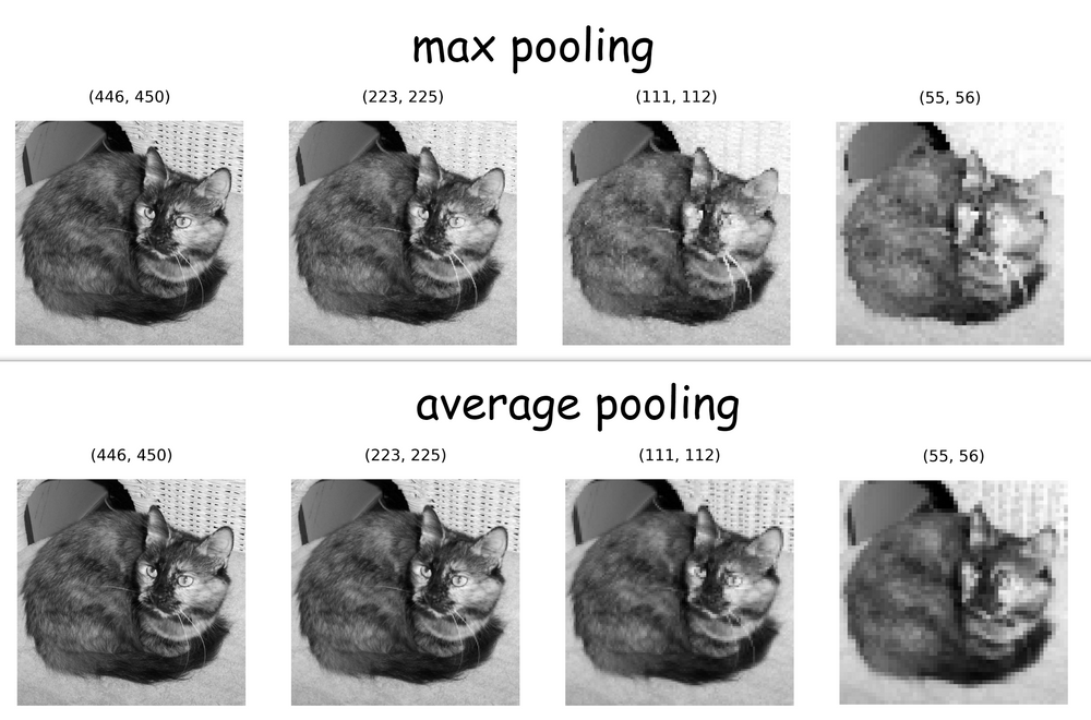
The pooling operation typically uses a 2x2 window with a stride of 2. This means it looks at a 2x2 block of pixels, calculates a single output value (the max or average), and then moves 2 pixels over to process the next block, with no overlap. The effect is that both the height and width of the feature map are halved, reducing the total number of values to 25% of the original!
Let's look at a visual comparison.
For a more hands-on feel of the calculation, the following resource provides a step-by-step walkthrough. This aligns with your preference for building mathematical understanding through practical examples.
A Gentle Introduction to Pooling Layers for Convolutional...
The article 'A Gentle Introduction to Pooling Layers' from Machine Learning Mastery walks through the manual calculation for both average and max pooling.
I recommend skimming the sections 'Average Pooling Layer' and 'Max Pooling Layer'. You don't need to read the code, but focus on the manual calculations that show how a 6x6 feature map is reduced to a 3x3 map. This will solidify your understanding of the mechanics.
Now that we understand what pooling is, let's explore its two primary roles.
2. Role 1: Dimensionality Reduction
The most immediate effect of pooling is reducing the spatial dimensions (height and width) of the feature maps. This is crucial for several reasons:
- Computational Efficiency: Smaller feature maps mean fewer parameters and computations for subsequent layers. This allows us to build deeper and more complex networks without the computational cost becoming unmanageable.
- Wider Receptive Field: By summarizing a 2x2 neighborhood into a single value, a neuron in the next layer that looks at this value is effectively "seeing" a larger region of the original input. This helps the network to aggregate features and learn more abstract, higher-level concepts as we go deeper.
The video we watched earlier has a fantastic visualization of this process.
What are Pooling Layers in Deep Neural Networks?
Let's return to the video from Deep Learning with Yacine to see dimensionality reduction in action.
Watch the segment from 02:05 to 03:03. Notice how after each pooling layer, the feature map becomes smaller, forcing the representation to become more compact while retaining the most important (salient) features of the car.
3. Role 2: Creating Translation Invariance
This is arguably the most important conceptual role of pooling. In the last lesson, we learned that convolutional layers are translation equivariant. This means if you shift the input (e.g., move a cat from the left to the right), the feature map also shifts. The representation of the cat is the same, but its location in the feature map changes.
For many tasks, like image classification, we don't care where the object is, only that it is present. We want the network's output to be robust to small shifts, rotations, or scaling. This property is called invariance.
Pooling layers help the network achieve local translation invariance. By taking the maximum value from a neighborhood, the network becomes less sensitive to the exact position of the feature within that neighborhood. If a feature shifts slightly but remains within the same pooling window, the output of the max-pooling operation will not change.
The image below provides a perfect illustration of this concept.

This robustness to small translations is a key reason why CNNs are so successful in object recognition tasks. Let's watch the final segment of the video for a narrated explanation of this idea.
What are Pooling Layers in Deep Neural Networks?
This final clip explains the concept of translation invariance and why it's so important for object detection.
Watch from 06:10 to 07:41. Focus on the distinction between the equivariance of convolutions and the invariance introduced by pooling.
Test your understanding!
You have a 14x14 feature map from a convolutional layer. A strong feature has produced an activation value of 8 at position (row=5, col=9). All neighboring activations are less than 5. You apply a 2x2 max pooling layer with a stride of 2.
- What will be the dimensions of the output feature map?
- The original activation at
(5, 9)is part of a pooling window that covers rows 4 & 5 and columns 8 & 9. What will be the value and position of the corresponding activation in the output map? (Assume row/column indices start at 0). - Now, imagine the input image was shifted slightly, and the strong feature activation moves from
(5, 9)to(4, 8). What happens to the output activation you calculated in the previous question?
Show answer
- Since the pooling is
2x2with a stride of2, it halves each dimension. The output feature map will be7x7. - The pooling window covers the input region from
(4, 8)to(5, 9). Since the max value in this window is 8 (at position(5, 9)), the output activation will be 8. The position of this output neuron corresponds to the top-left corner of the window divided by the stride:row = 4 / 2 = 2,col = 8 / 2 = 4. So the output is at(2, 4). - The new activation at
(4, 8)is still within the same pooling window(4, 8)to(5, 9). The maximum value in that window is still 8. Therefore, the output activation at(2, 4)remains 8. The output is invariant to this small local shift.
Conclusion
Today, we've uncovered the simple yet powerful mechanism of pooling layers. While convolutional layers do the heavy lifting of feature extraction, pooling layers play a critical supporting role by refining the feature maps.
Key Takeaways:
- Pooling layers are typically placed after convolutional layers to downsample feature maps. They have no learnable parameters.
- Max Pooling is the most common type, selecting the strongest feature response in a local region.
- The first key role of pooling is dimensionality reduction. This reduces computational load and helps subsequent layers learn more global features by increasing their effective receptive field.
- The second key role is creating local translation invariance. This makes the model more robust to small shifts in the input data, which is essential for tasks like object recognition.
Preview of the Next Lesson:
We now understand the two main workhorses of a CNN's feature extraction block: convolutional layers for finding features and pooling layers for making the representations compact and robust. In the next lesson, we will finally put all the pieces together and assemble a basic Convolutional Neural Network from scratch to perform an image classification task.