Bayes' Theorem: Priors and Posteriors

1. The Vocabulary of Belief Updating

Before diving into statistical models, let's first build an intuition for the key terms. Bayes' theorem gives us a language for updating beliefs.

The video beautifully illustrates the three core components of Bayesian reasoning:

• Prior: Your initial belief before seeing new evidence. In the example, this was the low probability of a person being a librarian in the general population (the "base rate").
• Likelihood: The probability of observing the evidence, given your hypothesis. This was the estimate of how likely the "meek and tidy" description was for a librarian versus a farmer.
• Posterior: Your updated belief after combining your prior and the likelihood. This was the final calculated probability that Steve was a librarian, given the description.

2. From Events to Model Parameters

Now, let's translate this from a single puzzle to the world of statistical modeling, which is our ultimate goal in machine learning. Instead of a hypothesis like "Steve is a librarian," we are interested in a model parameter, which we'll call $\theta$. This $\theta$ could be the fairness of a coin, a coefficient in a regression model, or the weight in a neural network.

Bayes' theorem for statistical inference is written as:

This is the same fundamental formula, just with new labels. Let's break it down.

Let's solidify those definitions:

• $P(\theta )$ — The Prior Distribution: This is no longer just a single probability but an entire probability distribution over all possible values of the parameter $\theta$. It represents our belief about $\theta$ before we see any data.
• $P(D|\theta )$ — The Likelihood: This function tells us how probable the observed data $D$ is for each possible value of $\theta$. This is the same likelihood function you encountered in Maximum Likelihood Estimation (MLE), and it's the component that brings information from the data into our analysis.
• $P(\theta |D)$ — The Posterior Distribution: This is the result we are looking for. It's a new probability distribution for $\theta$ that represents our updated belief after observing the data. It is a principled compromise between our prior belief and the evidence from the data.
• $P(D)$ — The Marginal Likelihood (or Evidence): This term represents the probability of observing the data, averaged over all possible values of $\theta$. For now, you can think of it as just a normalization constant that ensures the posterior distribution integrates to 1. This is why the relationship is often written as a proportionality:

3. Specifying Priors and Posteriors in Practice

Let's make this concrete with a classic example: estimating the bias of a coin, $\theta$, which is the probability of getting heads. Let's say we flip the coin $n$ times and observe $S$ heads.

To perform a Bayesian analysis, we must specify the Prior and the Likelihood. The Posterior will then be derived from them.

As the article explains:

1. Prior Specification: Our parameter $\theta$ is a probability, so it must be between 0 and 1. The Beta distribution is a flexible probability distribution defined on the interval $[0,1]$. It is controlled by two parameters, $\alpha$ and $\beta$.

   • A Beta(1, 1) prior is a uniform distribution, representing an uninformative prior where we believe all values of $\theta$ are equally likely.
   • A Beta(30, 30) prior would be sharply peaked around 0.5, representing a strong informative prior that the coin is fair.

2. Likelihood Specification: The process of getting $S$ successes in $n$ independent trials is modeled by the Binomial distribution. So, our likelihood function is $P(D|\theta )\propto {\theta }^S(1-\theta {)}^{n-S}$.

3. Posterior Derivation: When we combine a Beta prior with a Binomial likelihood, something mathematically convenient happens.

   • Prior: $P(\theta )\propto {\theta }^{\alpha -1}(1-\theta {)}^{\beta -1}$
   • Likelihood: $P(D|\theta )\propto {\theta }^S(1-\theta {)}^{n-S}$
   • Posterior: $P(\theta |D)\propto \text{Likelihood}\times \text{Prior}$ $$P(\theta |D)\propto \left({\theta }^S(1-\theta {)}^{n-S}\right)\times \left({\theta }^{\alpha -1}(1-\theta {)}^{\beta -1}\right)$$ $$P(\theta |D)\propto {\theta }^{S+\alpha -1}(1-\theta {)}^{n-S+\beta -1}$$

   This resulting expression has the exact form of another Beta distribution! Our posterior distribution is:

   $$\theta |D\sim \text{Beta}({\alpha }^{\prime }=\alpha +S,{\beta }^{\prime }=\beta +n-S)$$

This is the core of the process. We specified a Beta prior, used a Binomial likelihood, and found that our posterior is also a Beta distribution with updated parameters. The update rule is simple and intuitive: we just add the number of observed successes ($S$) to $\alpha$ and the number of observed failures ($n-S$) to $\beta$.

4. Visualizing the Belief Update

The power of this approach is seeing how our belief distribution changes as we incorporate data.

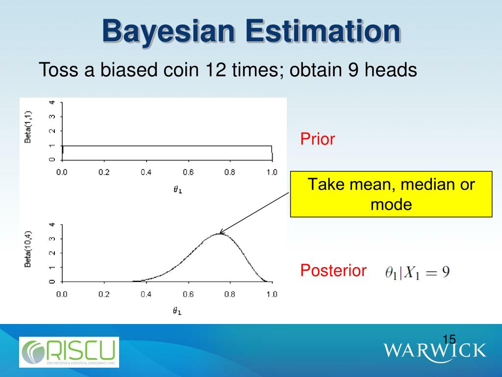
As we collect more and more data, the likelihood starts to dominate the prior. Our posterior distribution becomes narrower and more peaked, reflecting our increasing certainty about the true value of the parameter.

Conclusion

In this lesson, we moved from the philosophy of Bayesianism to its practice. We've seen how to formally set up a Bayesian analysis by specifying distributions that represent our beliefs and our model of the data.

Key Takeaways:

• Bayesian inference uses the language of distributions to represent beliefs about model parameters.
• The prior distribution $P(\theta )$ quantifies our belief about a parameter before seeing data. It can be informative (based on past knowledge) or uninformative (reflecting ignorance).
• The posterior distribution $P(\theta |D)$ represents our updated belief after seeing data. It is the central result of a Bayesian analysis.
• The posterior is calculated by combining the prior and the likelihood: Posterior $\propto$ Likelihood $\times$ Prior.
• In the Beta-Binomial model, the update from prior to posterior is a simple matter of adding observed counts to the prior's parameters.

Preview of the Next Lesson:

The mathematical convenience we saw with the Beta-Binomial model—where the posterior ends up in the same family as the prior—is a special and very important property. In the next lesson, we will explore this concept in more detail, formally defining conjugate priors and explaining their crucial role in simplifying Bayesian computation.