Bias-Variance Tradeoff and Model Complexity

The Core Tension: Underfitting vs. Overfitting

Imagine trying to predict a mouse's height from its weight. The true relationship is probably a curve—mice get taller as they get heavier, but only up to a point.

1. A Simple Model (High Bias): If we try to fit a straight line to this curved data, our model is too simple. It can't capture the true relationship, no matter how much data we give it. This failure to capture the underlying pattern is called bias. A high-bias model underfits the data.
2. A Complex Model (High Variance): Now, imagine we use an extremely "flexible" or "squiggly" line that perfectly weaves through every single data point in our training set. This model might have zero error on the data it was trained on, but it has likely memorized the random noise as well as the signal. When we show it new, unseen data, it will probably perform very poorly because it's too sensitive to the specific training set it saw. This sensitivity to the training data is called variance. A high-variance model overfits the data.

To build a solid intuition for this, let's watch a classic explanation from StatQuest.

As the video shows, the goal isn't to have zero training error. The goal is to build a model that generalizes well to new, unseen data. This requires finding a "sweet spot" between a model that's too simple (high bias) and one that's too complex (high variance).

This is the essence of the bias-variance tradeoff.

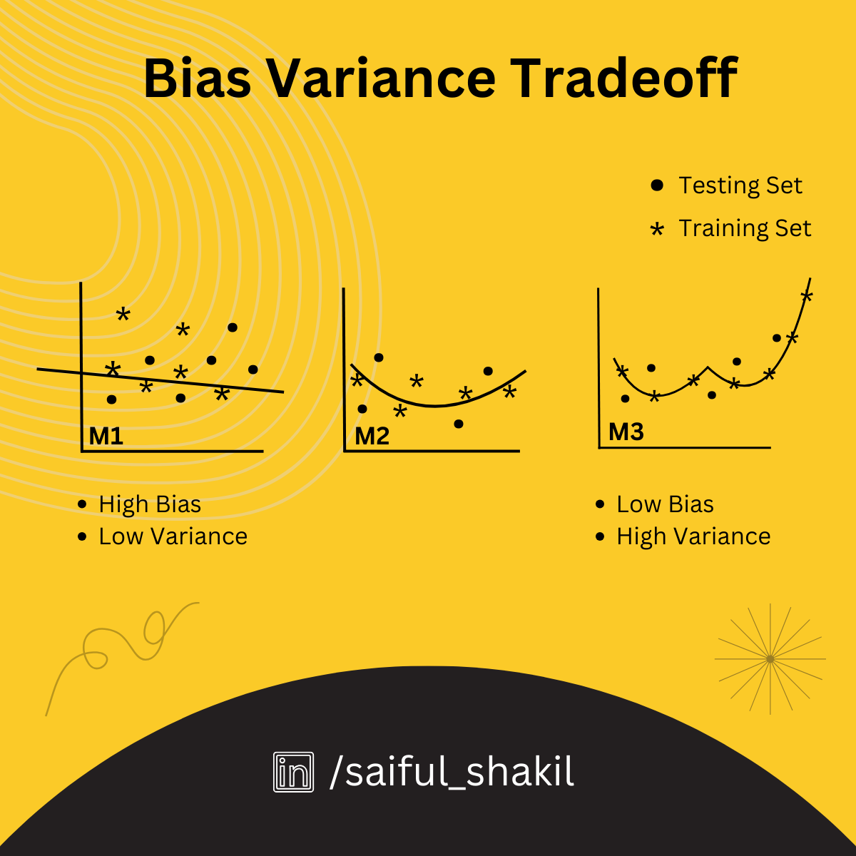
This image shows three models of increasing complexity. Model M1 (left) is too simple and underfits (high bias). Model M3 (right) is too complex and overfits the training data (high variance). Model M2 (center) strikes a good balance.

Decomposing a Model's Error

To move beyond intuition, we can mathematically formalize this concept. The total expected error of any machine learning model on unseen data can be decomposed into three components:

Let's break these down:

• Bias²: This term represents the error from the model's simplifying assumptions. It's a measure of how far off the average prediction is from the true value. A high-bias model is systematically wrong in the same way, like a broken clock that's always 10 minutes slow.
• Variance: This term represents the model's sensitivity to the specific training data. It measures how much the model's predictions would "jump around" if we trained it on different subsets of our data. A high-variance model gives very different predictions depending on the exact data it was trained on.
• Irreducible Error: This term is the inherent noise or randomness in the data itself. Even a "perfect" model can't eliminate this error. It represents the lower bound on the error that any model can achieve.

To see this decomposition explained in a more formal but still accessible way, let's turn to a lecture from Stanford University.

A great visual analogy for bias and variance is a target (bulls-eye).

*This cheat sheet provides a compact summary. The target diagrams on the top left are especially useful:

• Low Bias, Low Variance (Top-Left): Predictions are accurate and consistent (the ideal).
• Low Bias, High Variance (Top-Right): Predictions are accurate on average but scattered (overfitting).
• High Bias, Low Variance (Bottom-Left): Predictions are consistent but systematically wrong (underfitting).
• High Bias, High Variance (Bottom-Right): Predictions are inaccurate and inconsistent (the worst case).*

The Tradeoff Curve and Model Complexity

As the Stanford video showed, bias and variance typically have an inverse relationship with respect to model complexity.

• As you increase model complexity (e.g., using a higher-degree polynomial, a deeper decision tree):

  • Bias decreases (the model can fit more intricate patterns).
  • Variance increases (the model becomes more likely to fit the noise in the training data).

• As you decrease model complexity:

  • Bias increases (the model's assumptions become too simple).
  • Variance decreases (the model is less sensitive to the training data).

This leads to the characteristic U-shaped curve for the total error on the test set. Our goal as machine learning engineers is to find the level of complexity at the bottom of that "U".

This graph shows how bias decreases and variance increases as model complexity grows. The total error on unseen data (the red curve) is minimized at an optimal point of complexity, balancing the two.

Seeing the Tradeoff in Practice with Code

Let's make this concrete. A common way to increase the complexity of a linear model is to use Polynomial Regression. Instead of just fitting a line $y={\beta }_0+{\beta }_{1}x$, we can fit a curve by adding polynomial terms: $y={\beta }_0+{\beta }_{1}x+{\beta }_2{x}^2+\dots$. The degree of the polynomial is our knob for controlling model complexity.

The following code demonstrates this perfectly. It tries to fit a noisy cosine wave using polynomials of different degrees.

import numpy as np
import matplotlib.pyplot as plt
from sklearn.pipeline import Pipeline
from sklearn.preprocessing import PolynomialFeatures
from sklearn.linear_model import LinearRegression
from sklearn.metrics import mean_squared_error

# 1. Generate synthetic data (True function: Cosine)
np.random.seed(0)
n_samples = 30
degrees = [1, 4, 15] # Linear (Simple), Optimal, High Degree (Complex)

X = np.sort(np.random.rand(n_samples))
y = np.cos(1.5 * np.pi * X) + np.random.randn(n_samples) * 0.1 # Add noise

X_test = np.linspace(0, 1, 100)
plt.figure(figsize=(14, 5))

for i, degree in enumerate(degrees):
    ax = plt.subplot(1, 3, i + 1)
    
    # Create pipeline: Polynomial Features -> Linear Regression
    polynomial_features = PolynomialFeatures(degree=degree, include_bias=False)
    linear_regression = LinearRegression()
    pipeline = Pipeline([
        ("polynomial_features", polynomial_features),
        ("linear_regression", linear_regression),
    ])
    
    # Train model
    pipeline.fit(X[:, np.newaxis], y)
    
    # Evaluate
    y_pred = pipeline.predict(X_test[:, np.newaxis])
    train_score = mean_squared_error(y, pipeline.predict(X[:, np.newaxis]))
    
    # Plotting
    plt.plot(X_test, y_pred, label=f"Model (Degree {degree})")
    plt.plot(X_test, np.cos(1.5 * np.pi * X_test), label="True Function", linestyle="--")
    plt.scatter(X, y, edgecolor='b', s=20, label="Training Data")
    plt.title(f"Degree {degree}\nMSE = {train_score:.2e}")
    plt.ylim(-1.5, 1.5)
    plt.legend(loc="best")

plt.show()

When you run this code, you'll see three plots:

1. Degree 1 (High Bias): A straight line that completely fails to capture the cosine curve. It has underfit the data.
2. Degree 4 (Good Balance): A curve that closely follows the true function, ignoring most of the random noise. This is near the "sweet spot".
3. Degree 15 (High Variance): A wild curve that wiggles violently to pass through almost every single training point. It has perfectly learned the training data, including the noise. This is severe overfitting.

This practical example encapsulates the entire tradeoff in one visual. To explore this further, I recommend reading through the following Kaggle notebook which not only visualizes this but also shows how to calculate the bias and variance values.

Conclusion

Today we've unpacked one of the most essential concepts in machine learning. The bias-variance tradeoff is the central challenge you will face in almost every modeling project. Your ability to diagnose whether your model is suffering from high bias or high variance and knowing how to correct it is a critical skill.

Key Takeaways:

• Bias is error from a model being too simple (underfitting). It's characterized by high error on both training and test data.
• Variance is error from a model being too complex and sensitive to noise (overfitting). It's characterized by very low error on training data but high error on test data.
• A model's total error is a sum of its Bias², Variance, and Irreducible Error.
• Increasing model complexity generally decreases bias but increases variance. The goal is to find the optimal complexity that minimizes the total error on unseen data.

Preview of the Next Lesson:

In our exercise, one of the key solutions for fixing a high-variance model was regularization. This is not just a theoretical idea; it's a powerful and practical technique. In our next lesson, we will dive into two of the most common types of regularization for linear models: Ridge (L2) and Lasso (L1) regularization. You'll learn how these methods mathematically penalize complexity to help us find that "sweet spot" in the bias-variance tradeoff.