L1 vs. L2 Penalties: Coefficient Impact

Why Does the Penalty's Shape Matter?

The difference between Lasso ($\sum |{\beta }_j|$) and Ridge ($\sum {\beta }_j^2$) lies in the mathematical shape of their penalty functions. This shape directly influences how the model's cost function is optimized and, consequently, how the final coefficients are determined.

Let's start by visualizing the penalty's effect on the cost function for a single coefficient.

• The original error (Sum of Squared Errors) is a smooth parabola.
• The L2 penalty ($\alpha {\beta }^2$) is also a smooth parabola. When you add two parabolas together, you get another smooth parabola. Its minimum will be shifted closer to zero, but it's very unlikely to be exactly at zero.
• The L1 penalty ($\alpha |\beta |$) is a 'V' shape. When you add this 'V' to the error parabola, the resulting cost function has a sharp "kink" at zero. This kink makes zero a special point for the optimization algorithm, and it's quite possible for the minimum of the overall function to land exactly there.

To see this in action, the following video provides an excellent visualization.

This "kink" is the mathematical reason for Lasso's sparsity. An optimizer searching for the minimum cost can "fall" into this kink, resulting in a coefficient of exactly zero.

The Geometric Interpretation: Budgets and Contours

A more intuitive way to understand this is through a geometric analogy. Imagine you are trying to minimize your model's error (Sum of Squared Errors, SSE), but you have a limited "budget" for your coefficients.

• The error can be visualized as a set of concentric elliptical contours. The center of the ellipses represents the un-regularized best solution (the OLS estimates, let's call it ${\hat{\beta }}_{\text{OLS}}$), and the goal is to get to the innermost contour possible.
• The regularization penalty defines the shape of your budget, also known as the constraint region. We can't let our coefficients go outside this region.
  • For Ridge (L2), the constraint $\sum {\beta }_j^2\le t$ forms a circle (in 2D) or a hypersphere (in higher dimensions).
  • For Lasso (L1), the constraint $\sum |{\beta }_j|\le t$ forms a diamond (in 2D) or a rhomboid shape (in higher dimensions).

The optimal regularized solution is the point where the error contours first touch the boundary of the constraint region.

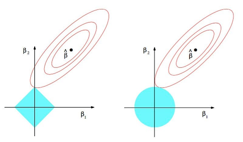
Look at the image above.

• With the L1 diamond, the sharp corners lie on the axes. It is highly probable that the expanding error ellipses will touch one of these corners first. When the solution lies on an axis (like at the top corner), the value of the other coefficient (${\beta }_1$) is exactly zero.
• With the L2 circle, the boundary is smooth. The error ellipse can touch the circle at any point. It's only by pure chance that this tangent point would lie exactly on an axis. The solution will almost always have non-zero values for both coefficients.

This geometric view is one of the most important intuitions in regularization. The following article provides a superb, detailed explanation.

Visualizing Coefficient Paths

We can summarize these effects by plotting the value of each coefficient as we increase the regularization strength ($\alpha$). These are called "coefficient paths."

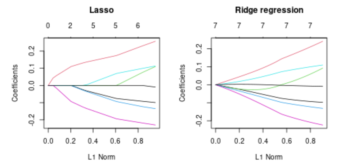
In this visualization, you can clearly see the concepts we've discussed:

• Lasso (Left): As the regularization gets stronger (moving from right to left on the x-axis), the coefficients are pulled towards zero. One by one, they hit zero and stay there. This is feature selection in action.
• Ridge (Right): The coefficients are also pulled towards zero, but they tend to shrink together and only approach zero asymptotically. They never quite reach it.

A Key Practical Difference: Handling Correlated Features

This difference in geometry and behavior has a very important practical implication when your dataset contains correlated features (multicollinearity).

Imagine you have two features that are nearly identical, like total_rooms and num_bedrooms in a housing dataset.

• Ridge Regression will tend to shrink the coefficients of these correlated features together. It gives them similar, non-zero coefficients, effectively "sharing the credit" between them. This makes the model more stable.
• Lasso Regression, due to its sharp geometry, will be somewhat "unstable" or "greedy." It will tend to arbitrarily pick one of the features, give it a non-zero coefficient, and shrink the other one completely to zero. Which one it picks can be almost random.

Conclusion

You now have a deep, intuitive understanding of not just what L1 and L2 regularization do, but why they behave so differently. This knowledge is crucial for making informed modeling decisions.

Key Takeaways:

• The L1 penalty (Lasso) corresponds to a diamond-shaped constraint region. Its sharp corners lie on the axes, making it highly likely that the optimal solution will have some coefficients that are exactly zero. This performs feature selection.
• The L2 penalty (Ridge) corresponds to a circular constraint region. Its smooth boundary means the optimal solution can be anywhere on the edge, making it highly unlikely that any coefficient will be exactly zero. It performs coefficient shrinkage.
• With correlated features, Ridge tends to shrink coefficients together, while Lasso will arbitrarily select one and eliminate the others.

Preview of the Next Lesson:

So, which is better? Lasso is great for feature selection, but Ridge is more stable with correlated features. What if we want the best of both worlds? In our next lesson, we will explore Elastic Net, a hybrid model that combines L1 and L2 penalties. We will also cover the essential practical skill of using k-fold cross-validation to find the optimal regularization strength, allowing you to tune your models for the best possible performance.