Expected Value and Variance of Random Variables

Hello! Welcome to your next lesson in our "Probability and Distributions for Modeling Data" module.

In our last session, we explored Bayes' theorem and saw how it allows us to update our beliefs about a model's parameters, resulting in a posterior probability distribution. This distribution represents everything we've learned from the data. But a full distribution can be unwieldy. How can we summarize its key characteristics?

Today, we'll answer that question by focusing on two of the most fundamental summary statistics. Our learning outcome is to calculate the expected value and variance of random variables to characterize their central tendency and spread. The expected value will give us a single "best guess" for our parameter, while the variance will tell us how uncertain we are about that guess.

1. The "Center of Mass": Understanding Expected Value

You're already familiar with the concept of the mean or average from descriptive statistics. The expected value, denoted $E [X]$ , is the probabilistic equivalent. It represents the long-run average value of a random variable if we were to repeat an experiment infinitely many times.

One powerful way to think about this comes from a concept that might be familiar from your engineering studies: moments. The expected value is the "first moment" of a probability distribution, which is conceptually similar to finding the center of mass of an object.

The following video provides an excellent intuition for this idea, framing the mean as the average distance of the data points from zero.

What are "moments" in statistics? An intuitive video!

Watch this segment from the zedstatistics channel to build an intuition for the mean as the 'first moment' of a distribution.

Watch the beginning of the video, from 00:00 to 04:04. Pay attention to how the concept of 'average distance from 0' is used to define the first moment, which is simply the mean.

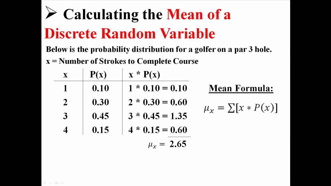
As the video illustrates, the mean gives us a measure of the distribution's center. Formally, for a discrete random variable $X$ that can take values $x_{1}, x_{2}, \dots, x_{n}$ with corresponding probabilities $P (X = x_{1}), P (X = x_{2}), \dots, P (X = x_{n})$ , the expected value is the probability-weighted sum of the possible values:

$E [X] = \sum_{i = 1}^{n} x_{i} \cdot P (X = x_{i})$

This is like a normal average, but instead of giving each value equal weight, we weight each value by its probability of occurring. The resource from Berkeley Statistics provides a clear definition and uses the analogy of a "balancing point" for the probability distribution.

Expected value and variance of a random variable

This resource reinforces the definition of expected value as a weighted average and introduces the 'balancing point' analogy.

Read the first section, 'Expectation of a random variable', up to the 'Properties of expectation' part. Focus on the formal definition and the examples with the fair and unfair dice.

The image below gives a simple, concrete example of this calculation.

Calculating the Mean of a Discrete Random Variable — This table shows the calculation of the expected value (mean) for a golfer's score on a par 3 hole. Each possible score `x` is multiplied by its probability `P(x)`, and these products are summed to find the overall expected score, $\mu_x = 3.05$.

2. The "Spread": Understanding Variance

The expected value tells us where the center of a distribution is, but it doesn't tell us anything about how spread out the values are. For example, two datasets could have the same mean but vastly different levels of dispersion.

This is where the concept of variance comes in. Variance measures the average squared difference of each value from the mean. We square the differences so that negative and positive deviations don't cancel each other out, and it also penalizes values that are further from the mean more heavily.

The video on "moments" that you started earlier has a brilliant explanation of how we arrive at variance by "centering" the data around the mean first. This leads to the "second centered moment," which is precisely the variance.

What are "moments" in statistics? An intuitive video!

Let's return to the 'moments' video to see how variance is developed as a measure of spread that is independent of the mean.

Watch the segment from 04:04 to 09:13. This part first explains the problem with the 'crude' second moment and then shows how subtracting the mean leads to the 'centered' second moment, or variance, which is a pure measure of spread.

The formal definition of variance, denoted $V a r (X)$ or $σ^{2}$ , is the expected value of the squared deviation from the mean $μ = E [X]$ :

$V a r (X) = E [(X - μ)^{2}] = \sum_{i = 1}^{n} (x_{i} - μ)^{2} \cdot P (X = x_{i})$

Because the units of variance are squared (e.g., dollars-squared), we often take its square root to get a measure of spread in the original units. This is called the standard deviation, denoted $σ$ .

$σ = V a r (X)$

3. How to Calculate Expected Value and Variance

Now let's see how these calculations work in practice. While the definitional formula for variance is intuitive, a different formula is often easier to use for calculations.

Computational Formula for Variance:
It can be shown that $E [(X - μ)^{2}]$ is mathematically equivalent to:
$V a r (X) = E [X^{2}] - (E [X])^{2}$
This is often called the shortcut or computational formula. To use it, you calculate two things:

$E [X]$ , the expected value of $X$ .
$E [X^{2}]$ , the expected value of $X^{2}$ , which is calculated as $\sum x_{i}^{2} \cdot P (X = x_{i})$ .

Then, you just plug them into the formula: $V a r (X) = E [X^{2}] - (E [X])^{2}$ .

The following video is an excellent, step-by-step guide to calculating both expected value and variance for a discrete random variable. It demonstrates the calculation of variance using both the definitional and computational formulas, showing they yield the same result.

The Expected Value and Variance of Discrete Random Variables

Watch this jbstatistics video for a clear, worked-out example of calculating E[X] and Var(X).

Please watch the following segments: Calculating Expected Value (04:27 - 06:24): Follow the calculation for the number of heads in a coin toss experiment. Calculating Variance (07:26 - 10:37): This is a key section. Pay close attention to how the narrator calculates the variance first using the definition E[(X-\mu)^2] and then verifies it using the computational formula E[X^2] - (E[X])^2. Recap (10:37 - 11:10): A quick summary of the two ways to calculate variance.

Test your understanding!

A random variable $Y$ represents the number of defects found in a product sample. Its probability distribution is given below:

$y$ (Defects)	$P (Y = y)$
0	0.7
1	0.2
2	0.1

Calculate the expected value $E [Y]$ and the variance $V a r (Y)$ .

Show answer

1. Calculate Expected Value $E [Y]$ :
$E [Y] = (0 \cdot 0.7) + (1 \cdot 0.2) + (2 \cdot 0.1)$
$E [Y] = 0 + 0.2 + 0.2 = 0.4$
The expected number of defects is 0.4.

2. Calculate Variance $V a r (Y)$ using the computational formula:
First, we need $E [Y^{2}]$ :
$E [Y^{2}] = (0^{2} \cdot 0.7) + (1^{2} \cdot 0.2) + (2^{2} \cdot 0.1)$
$E [Y^{2}] = (0 \cdot 0.7) + (1 \cdot 0.2) + (4 \cdot 0.1)$
$E [Y^{2}] = 0 + 0.2 + 0.4 = 0.6$

Now, use the formula $V a r (Y) = E [Y^{2}] - (E [Y])^{2}$ :
$V a r (Y) = 0.6 - (0.4)^{2}$
$V a r (Y) = 0.6 - 0.16 = 0.44$
The variance of the number of defects is 0.44.

4. From Theory to Practice with Python

In machine learning, we don't usually know the true probability distribution. Instead, we have a sample of data that we assume is drawn from that distribution. We can then calculate the sample mean and sample variance from our data to estimate the true expected value and variance.

Given your goal of applying statistics to ML, it's useful to see how this is done in code.

A Gentle Introduction to Expected Value, Variance, and ...

This article from Machine Learning Mastery connects the statistical theory to practical Python code using the NumPy library.

Read the sections 'Expected Value' and 'Variance'. Notice how numpy.mean() and numpy.var() are used to calculate these statistics from a sample of data. The var() function discusses the ddof argument, which is a small correction used when estimating variance from a sample instead of a full population. We'll delve deeper into this distinction in a future module on statistical inference.

Conclusion

Today, we've established how to summarize probability distributions using two key numbers. We've seen that expected value and variance aren't just abstract formulas; they are the first and second "moments" that describe a distribution's center and spread.

Key Takeaways:

Expected Value $E [X]$ is the probability-weighted average of a random variable's possible outcomes. It tells us the distribution's center of mass or long-run average.
Variance $V a r (X)$ is the expected squared deviation from the mean, $E [(X - μ)^{2}]$ . It measures the spread or dispersion of the distribution.
The Standard Deviation ( $σ$ ) is the square root of the variance and provides a measure of spread in the original units of the data.
The computational formula for variance, $V a r (X) = E [X^{2}] - (E [X])^{2}$ , is often the most practical way to perform the calculation.

Next Steps:
Now that you know how to characterize any random variable by its mean and variance, we are ready to study some specific, named probability distributions that appear constantly in machine learning. In the next lesson, we will begin with distributions used for modeling binary outcomes and counts: the Bernoulli, Binomial, and Poisson distributions. We will see how to apply the concepts from today to find their specific expected values and variances.

Recommended resources

1. The "Center of Mass": Understanding Expected Value

2. The "Spread": Understanding Variance

3. How to Calculate Expected Value and Variance

4. From Theory to Practice with Python

Conclusion