Hello! Welcome to the next lesson in your journey to master statistics for machine learning.
In our last lesson, we saw how to generalize logistic regression from two classes to many using the powerful softmax function. We can now build classifiers for complex problems like identifying different types of objects in images or categorizing news articles. But building a model is only half the battle. How do we know if it's actually any good?
You might think to use accuracy—the percentage of correct predictions. However, as we'll see, accuracy can be dangerously misleading, especially when dealing with real-world data where some outcomes are much rarer than others.
Today, we'll dive into a more robust toolkit for evaluating your classification models. Our goal is to evaluate a classifier's performance using a confusion matrix, precision, recall, and F1-score. These metrics will give you a much deeper, more nuanced understanding of your model's strengths and weaknesses, allowing you to justify why one model is better than another for a specific task.
Why Accuracy Is Not Enough
Imagine you're building a model to detect fraudulent credit card transactions. Fraud is rare; let's say only 0.1% of transactions are actually fraudulent. A lazy model that simply predicts "not fraud" for every single transaction would achieve 99.9% accuracy! It sounds impressive, but it's completely useless because it fails to catch any fraud at all. This is an example of a class imbalance problem, and it highlights why we need better tools.
Beyond Accuracy: A Deep Dive into Classification Metrics
This article, 'Beyond Accuracy', starts by reinforcing this exact point and then introduces the foundation for our entire lesson: the Confusion Matrix.
Read the introductory section and the sections titled 'The Confusion Matrix: The Foundation of Metrics' and 'Metric 1: Accuracy'. Focus on: The disease detection example that illustrates the limits of accuracy. The definitions of True Positive (TP), True Negative (TN), False Positive (FP), and False Negative (FN). When accuracy can be used, and more importantly, when it should not be used.
The Confusion Matrix: Deconstructing Model Performance
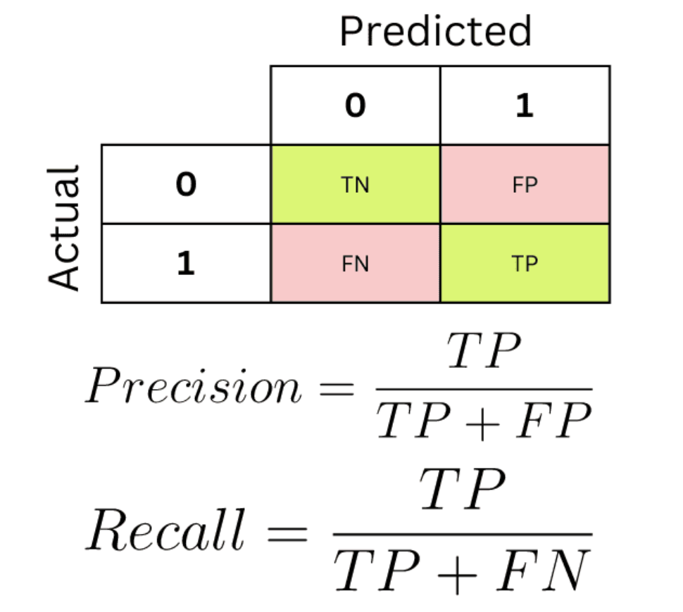
As you just read, the confusion matrix is the starting point for almost all classification metrics. It’s a simple table that breaks down how many times your model's predictions were right and wrong, and importantly, what kind of wrong they were.
Let's get a more visual and detailed walkthrough of how to build and interpret one.
Making sense of the confusion matrix
This video from Data School provides an excellent, step-by-step explanation of the confusion matrix.
Please watch from the beginning to 07:32. Pay close attention to: The definition of a confusion matrix and when it's used. How to read the 2x2 matrix layout (Actual vs. Predicted). The meaning of the four cells: True Positives, True Negatives, False Positives (Type I Error), and False Negatives (Type II Error).
To summarize the key terms:
- True Positive (TP): Correctly predicted positive. (e.g., Model says "disease," patient has disease).
- True Negative (TN): Correctly predicted negative. (e.g., Model says "no disease," patient is healthy).
- False Positive (FP): Incorrectly predicted positive. A "false alarm." (e.g., Model says "disease," but patient is healthy). This is a Type I Error.
- False Negative (FN): Incorrectly predicted negative. A "miss." (e.g., Model says "no disease," but patient has disease). This is a Type II Error.
Precision and Recall: The Two Pillars of Evaluation
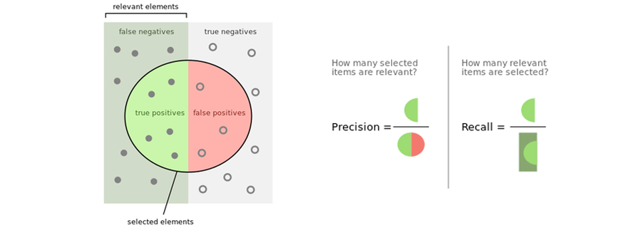
Now that we have the counts from the confusion matrix, we can calculate more insightful metrics. Two of the most important are Precision and Recall. They measure two different aspects of a model's performance and often exist in a trade-off.
Precision: How Trustworthy Are the Positive Predictions?
Precision answers the question: "Of all the instances the model predicted as positive, how many were actually positive?"
- High Precision means that when your model predicts a positive outcome, it is very likely to be correct.
- The goal of maximizing precision is to minimize False Positives (FP).
Recall: How Well Did We Find All the Positives?
Recall (also known as Sensitivity or True Positive Rate) answers the question: "Of all the instances that were actually positive, how many did the model correctly identify?"
- High Recall means that your model is good at finding all the positive instances in your dataset.
- The goal of maximizing recall is to minimize False Negatives (FN).
For a very intuitive and memorable explanation of this trade-off, the following short video uses great analogies.
MFML 044 - Precision vs recall
Cassie Kozyrkov from Google uses two fun scenarios—a book recommender and robbing a house—to illustrate when you would care more about precision versus recall.
Watch from 02:29 to 05:40. Think about why a 'precision mindset' is right for book recommendations and a 'recall mindset' is right for collecting jewelry.
Context is King: Choosing Between Precision and Recall
As you've seen, the "best" metric depends entirely on your business objective. The key is to analyze the cost of each type of error.
Beyond Accuracy: A Deep Dive into Classification Metrics
Let's revisit the 'Beyond Accuracy' article to solidify our understanding of when to use each metric.
Read the sections 'Metric 2: Precision (Minimizing False Positives)' and 'Metric 3: Recall (Minimizing False Negatives)'. The examples provided are classic scenarios you'll encounter in ML interviews and real-world projects.
Let's summarize the key scenarios:
- Prioritize High Precision when the cost of a False Positive is high.
- Spam Filter: You would rather have a few spam emails get into your inbox (False Negative) than have an important email sent to your spam folder (False Positive).
- Legal Evidence: Falsely identifying someone as guilty (False Positive) has extreme consequences.
- Prioritize High Recall when the cost of a False Negative is high.
- Cancer Diagnosis: It's far better to have a false alarm and run more tests (False Positive) than to miss an actual case of cancer (False Negative).
- Fraud Detection: A bank would rather temporarily flag a legitimate transaction for verification (False Positive) than let a fraudulent one go through unnoticed (False Negative).
Test your understanding!
You are tasked with building a model for an airport security scanner to automatically detect prohibited items (like weapons) in luggage. Would you design the system to prioritize high precision or high recall? Explain your reasoning in terms of False Positives and False Negatives.
Show answer
You would prioritize high recall.
- A False Negative in this context means a prohibited item was in a bag, but the system failed to flag it. This is a massive security risk and has catastrophic consequences. We must minimize these misses.
- A False Positive means a harmless item was flagged as prohibited, requiring a manual inspection by a security officer. While this is an inconvenience, it is far more acceptable than the alternative.
Therefore, the system should be optimized for recall to ensure it "recalls" or catches as many actual prohibited items as possible, even if it means generating more false alarms.
The F1-Score: A Single Metric to Rule Them All?
What if both precision and recall are important? Or what if you just want a single number to compare different models? This is where the F1-Score comes in.
The F1-Score is the harmonic mean of precision and recall.
The use of the harmonic mean is deliberate. Unlike a simple average, it heavily penalizes low scores. If either precision or recall is close to zero, the F1-score will also be close to zero. A model must have reasonably high precision and recall to get a high F1-score. This makes it a more balanced and reliable metric than accuracy, especially on imbalanced datasets.
Beyond Accuracy: A Deep Dive into Classification Metrics
The 'Beyond Accuracy' article has a concise section on the F1-Score.
Read the section titled 'Metric 4: F1-Score (Balancing Precision and Recall)' to understand its definition and when it's most useful.
From Theory to Practice: A Worked Example
Let's tie all these concepts together. Imagine we have a classifier trying to identify dog images. We test it on 10 images and get the following results:
| Image | 1 | 2 | 3 | 4 | 5 | 6 | 7 | 8 | 9 | 10 |
|---|---|---|---|---|---|---|---|---|---|---|
| Actual | Dog | Dog | Dog | Not Dog | Dog | Not Dog | Dog | Dog | Not Dog | Not Dog |
| Predicted | Dog | Not Dog | Dog | Not Dog | Dog | Dog | Dog | Dog | Not Dog | Not Dog |
First, let's build the confusion matrix. We define "Dog" as our positive class.
- TP: Actual is 'Dog', Predicted is 'Dog' = 5
- FN: Actual is 'Dog', Predicted is 'Not Dog' = 1
- FP: Actual is 'Not Dog', Predicted is 'Dog' = 1
- TN: Actual is 'Not Dog', Predicted is 'Not Dog' = 3
Our confusion matrix is:
| Predicted: Dog | Predicted: Not Dog | |
|---|---|---|
| Actual: Dog | 5 (TP) | 1 (FN) |
| Actual: Not Dog | 1 (FP) | 3 (TN) |
Now we can calculate our metrics:
- Accuracy: (80%)
- Precision: (83.3%)
- Recall: (83.3%)
- F1-Score: (83.3%)
In practice, you won't do this by hand. Libraries like scikit-learn provide functions that do it all for you.
Understanding the Confusion Matrix in Machine Learning
This GeeksForGeeks article provides a simple Python implementation that reproduces this exact example and shows the output of scikit-learn's classification_report.
Read the sections 'Confusion Matrix For Binary Classification' and 'Implementation of Confusion Matrix for Binary classification using Python'. You don't need to run the code, but observe how the code generates the confusion matrix and a classification_report containing precision, recall, and f1-score automatically.
The classification_report also shows you how these metrics can be calculated for each class individually, which is exactly how we evaluate the multi-class classifiers we learned about in the previous lesson. The process is simply repeated for each class in a one-vs-rest manner.
Conclusion
You've now added a critical set of tools to your model evaluation toolbox. You've moved beyond simple accuracy to a more sophisticated understanding of classifier performance.
Key Takeaways:
- Accuracy is misleading for imbalanced datasets.
- The Confusion Matrix is the foundation for evaluation, breaking down predictions into True/False Positives and True/False Negatives.
- Precision measures the quality of positive predictions (minimizing FP), crucial when false alarms are costly.
- Recall measures the completeness of positive predictions (minimizing FN), crucial when misses are costly.
- The F1-Score provides a single, balanced metric by calculating the harmonic mean of precision and recall.
- The choice of metric is not a technical decision alone; it must be driven by the business context and the cost of different errors.
Preview of the Next Lesson:
Our calculations for precision and recall were based on the final "yes" or "no" predictions. But remember, a logistic regression model outputs a probability (e.g., 0.75). We get a final prediction by applying a threshold (e.g., if probability > 0.5, predict "yes"). What happens if we change that threshold? How does that affect our precision and recall?
In the next lesson, we will construct and interpret a Receiver Operating Characteristic (ROC) curve and the Area Under the Curve (AUC). These powerful tools allow us to evaluate a model's performance across all possible thresholds, giving us a complete, threshold-independent view of its predictive power.