SVMs: Intuition and Margin Maximization

Part 1: The Core Idea - Maximal Margin Classification

Imagine you have a dataset with two classes that are clearly separable. You could draw many different lines (or "hyperplanes") to separate them. But which one is the best?

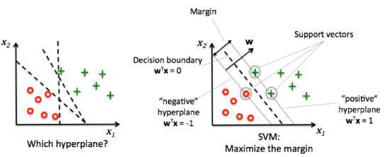
The core intuition of an SVM is to choose the hyperplane that is as far as possible from the nearest data points of both classes. This is called margin maximization.

Think of it like this: you're a construction company tasked with building the widest possible straight highway between two cities (the two classes), where the buildings are your data points. The edges of your highway are determined by the buildings closest to the road. These critical buildings are the support vectors because they "support" or define the position of your highway. The width of the highway is the margin. An SVM aims to make this margin as wide as possible.

The line running down the middle of this highway is our decision boundary, called the hyperplane.

Let's watch a video that brings this concept to life.

This idealized version of finding the widest possible margin that perfectly separates the data is called a Hard Margin Classifier or a Maximal Margin Classifier. It's defined by three key terms:

• Hyperplane: The decision boundary (a line in 2D, a plane in 3D).
• Support Vectors: The data points closest to the hyperplane that dictate its position and orientation.
• Margin: The distance between the hyperplane and the support vectors. SVMs work by maximizing this.

Part 2: Dealing with Reality - The Soft Margin

The hard margin approach works beautifully for perfectly clean, linearly separable data. But real-world data is rarely so neat. What happens if there are outliers, or the classes overlap slightly?

A hard margin classifier is extremely sensitive to outliers. A single outlier can dramatically change the hyperplane and result in a much smaller margin, leading to a model that doesn't generalize well. This is an example of the bias-variance tradeoff: the hard margin model has high variance because it's so sensitive to the specific training data.

To create a more robust model, we can relax the rule that every data point must be outside the margin. This is the idea behind a Soft Margin Classifier.

A soft margin classifier allows some data points to be on the wrong side of the margin, or even on the wrong side of the hyperplane. It makes a tradeoff: it accepts a few errors on the training data in exchange for a wider, more stable margin that will likely perform better on new, unseen data.

How do we control this tradeoff? We use a hyperparameter, typically denoted as C.

To summarize the role of C:

• C is the regularization parameter that controls the penalty for misclassification.
• High C: Imposes a high penalty for misclassified points. The SVM will try to minimize errors, resulting in a narrower margin. This can lead to overfitting (high variance).
• Low C: Imposes a low penalty. The SVM is more tolerant of errors, allowing it to focus on finding a wider margin. This can lead to underfitting (high bias).

Choosing the right value for C is key to building a good SVM model and is usually done using techniques like cross-validation.

Part 3: Unleashing the Power of SVMs - The Kernel Trick

So far, we've only discussed linear boundaries. But what if the data is not linearly separable at all? Imagine one class forming a circle of points inside a ring of points from the other class. No straight line can separate them.

This is where SVMs truly shine, using a concept called the kernel trick.

The intuition is simple: if we can't separate the data in its current dimension, we can project it into a higher dimension where it becomes linearly separable.

The "trick" in the kernel trick is that we don't need to perform the computationally expensive step of actually creating these new dimensions. A kernel function allows us to calculate the dot products (which represent the relationships) between the data points as if they were in the higher-dimensional space.

This allows SVMs to create incredibly complex, non-linear decision boundaries efficiently. Common kernels include:

• Polynomial Kernel: Creates polynomial decision boundaries.
• Radial Basis Function (RBF) Kernel: Creates complex, localized boundaries. It is one of the most popular and powerful kernels.

A Glimpse Under the Hood

To tie these ideas together, let's briefly look at what the SVM algorithm is trying to optimize. You don't need to memorize the math, but seeing the objective function can clarify the concepts we've discussed.

The SVM is solving an optimization problem with two competing goals:

1. Maximize the margin. Mathematically, this is equivalent to minimizing ||w||², where w is the vector perpendicular to the hyperplane. A smaller w means a larger margin.
2. Minimize the number of margin violations. This is the sum of the errors (ζᵢ, or "slack variables") for each point that falls inside the margin or on the wrong side.

The final objective function looks like this:

${\min }_{w,b,\zeta }\frac{1}{2}||w|{|}^2+C{\sum }_{i=1}^m{\zeta }_i$

This equation perfectly captures the tradeoff:

• The first term (||w||²) pushes for a larger margin.
• The second term (C * Σζᵢ) pushes for fewer misclassifications.
• The hyperparameter C is the knob that balances these two competing goals.

This provides a concrete mathematical basis for the intuitive ideas of margin maximization and the soft margin tradeoff.

Conclusion

You now have a solid intuition for one of the most elegant and powerful classifiers in machine learning. Unlike logistic regression, which thinks in terms of probabilities, SVMs think in terms of geometric separation.

Key Takeaways:

• Support Vector Machines (SVMs) aim to find the optimal hyperplane that best separates classes.
• The core principle is margin maximization: finding the hyperplane that creates the widest possible "street" between the classes.
• Support vectors are the critical data points lying on the edge of the margin that define the hyperplane.
• Soft margins are used for real-world data, allowing some misclassifications to achieve a more robust, generalizable model. The C parameter controls this bias-variance tradeoff.
• The kernel trick is the key to applying SVMs to non-linear problems by implicitly projecting data into a higher dimension where it becomes linearly separable.

Preview of the Next Lesson:
In our next lesson, we will tackle a common practical challenge in classification: class imbalance. We'll learn how to diagnose when our dataset has a skewed distribution of classes and apply techniques like resampling and class weighting to ensure our models learn effectively. You'll see how the C parameter in SVMs can be adjusted to directly address this problem, providing a nice link back to today's topic.