Feynman Rules for Quartic Perturbation

Perturbation Theory for Correlation Functions

Let's begin with the full Landau-Ginzburg action, separated into its free and interacting parts:

where $S_0[\varphi ]=\int d^{d}x\left[\frac{1}{2}(\nabla \varphi {)}^2+\frac{r}{2}{\varphi }^2\right]$ is the free or Gaussian action, and $S_{int}[\varphi ]=\int d^{d}x\frac{u}{4!}{\varphi }^4(x)$ is the interaction term. The factor of $1/4!$ is a convention that will simplify our results by cancelling combinatorial factors later on.

The $n$-point correlation function in the interacting theory is given by the ratio of two functional integrals:

Since $u$ is assumed to be small, we can expand the term $e^{-S_{int}[\varphi ]}$ in a Taylor series:

Substituting this into the expression for the correlation function turns the problem into one of calculating expectation values in the free theory, which we denote by $⟨\dots {⟩}_0$. These are precisely the Gaussian averages that Wick's theorem allows us to compute.

Let's apply this to the two-point function, $⟨\varphi (x_1)\varphi (x_2)⟩$, keeping terms up to first order in $u$. The numerator (Num) and denominator (Den) become:
\begin{align*}
\text{Num} &= \int \mathcal{D}\phi , \phi(x_1)\phi(x_2) \left(1 - \frac{u}{4!} \int d^dy , \phi^4(y)\right) e^{-S_0} \
&= \langle \phi(x_1)\phi(x_2) \rangle_0 - \frac{u}{4!} \int d^dy , \langle \phi(x_1)\phi(x_2)\phi^4(y) \rangle_0 \
\text{Den} &= \int \mathcal{D}\phi , \left(1 - \frac{u}{4!} \int d^dy , \phi^4(y)\right) e^{-S_0} \
&= 1 - \frac{u}{4!} \int d^dy , \langle \phi^4(y) \rangle_0
\end{align*}
Note that we have normalized by $Z_0=\int \mathcal{D}\varphi e^{-S_0}$ to define the free-theory averages $⟨\dots {⟩}_0$.

The full two-point function is the ratio $\text{Num}/\text{Den}$. Using the approximation $1/(1-x)\approx 1+x$, we get:

Multiplying this out and keeping terms to $O(u)$ gives:

This central result tells us that the first-order correction is determined by the difference between a six-point and a four-point Gaussian average. This difference has a special name: the connected correlation function.

Wick's Theorem and the Birth of Diagrams

Now we must evaluate the Gaussian averages using Wick's theorem. Let's represent the bare propagator $⟨\varphi (x)\varphi (y){⟩}_0=G_0(x-y)$ by a simple line connecting points $x$ and $y$.

1. The Four-Point Average $⟨{\varphi }^4(y){⟩}_0$

We need to calculate $⟨\varphi (y)\varphi (y)\varphi (y)\varphi (y){⟩}_0$. Wick's theorem instructs us to sum over all pairings. There are $(4-1)!!=3$ ways to pair the four fields:

Diagrammatically, we represent the interaction vertex at point $y$ with a dot. The pairings correspond to lines originating and ending at this vertex. Since we have two propagators $G_0(0)$, we draw two loops. The three terms are topologically identical.

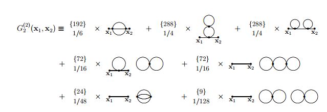
The term $G_0(0)$ is the propagator from a point back to itself, forming a loop. The term $⟨{\varphi }^4(y){⟩}_0$ is represented by two such loops emerging from the same interaction vertex $y$.

2. The Six-Point Average $⟨\varphi (x_1)\varphi (x_2){\varphi }^4(y){⟩}_0$

This is the expectation value of $\varphi (x_1)\varphi (x_2)\varphi (y)\varphi (y)\varphi (y)\varphi (y)$. Wick's theorem gives $(6-1)!!=15$ terms. We can group them by their graphical structure:

• Type 1: Disconnected diagrams. We pair $\varphi (x_1)$ with $\varphi (x_2)$ and pair the four $\varphi (y)$ fields among themselves.

  • The pairing of $\varphi (x_1)$ and $\varphi (x_2)$ gives one factor of $G_0(x_1-x_2)$.
  • The remaining $⟨{\varphi }^4(y){⟩}_0$ gives a factor of $3G_0(0{)}^2$.
  • The total contribution from these pairings is $3G_0(x_1-x_2)G_0(0{)}^2$.
  • Diagrammatically, this is a propagator from $x_1$ to $x_2$ that is completely separate from the double-loop diagram at vertex $y$.

• Type 2: Connected diagrams. We pair the "external" fields $\varphi (x_1)$ and $\varphi (x_2)$ with the "internal" fields at the interaction vertex $y$. For example, pair $\varphi (x_1)$ with a $\varphi (y)$, $\varphi (x_2)$ with another $\varphi (y)$, and the remaining two $\varphi (y)$'s with each other.

  • This gives a product of propagators: $G_0(x_1-y)G_0(x_2-y)G_0(y-y)$.
  • How many ways can we form this? There are 4 choices for which $\varphi (y)$ to pair with $\varphi (x_1)$, 3 choices for which to pair with $\varphi (x_2)$, and the last two $\varphi (y)$'s have 1 way to be paired. This gives $4\times 3\times 1=12$ identical terms.
  • The total contribution is $12G_0(x_1-y)G_0(x_2-y)G_0(0)$.
  • Diagrammatically, this corresponds to a line from $x_1$ to $y$, a line from $x_2$ to $y$, and a loop from $y$ back to itself. This is often called a "tadpole" diagram.

The Linked Cluster Theorem and Feynman Rules

Now, let's substitute these results back into our expression for the two-point function:
\begin{align*}
\langle \phi(x_1)\phi(x_2) \rangle &\approx G_0(x_1-x_2) - \frac{u}{4!} \int d^dy \left[ (3 G_0(x_1-x_2)G_0(0)^2 + 12 G_0(x_1-y)G_0(x_2-y)G_0(0)) - (G_0(x_1-x_2) \cdot 3 G_0(0)^2) \right] \
&= G_0(x_1-x_2) - \frac{12u}{24} \int d^dy , G_0(x_1-y)G_0(y-y)G_0(y-x_2) \
&= G_0(x_1-x_2) - \frac{u}{2} \int d^dy , G_0(x_1-y)G_0(0)G_0(y-x_2)
\end{align*}
Notice a remarkable cancellation: the disconnected part of the six-point function, $3G_0(x_1-x_2)G_0(0{)}^2$, is exactly cancelled by the term involving $⟨\varphi (x_1)\varphi (x_2){⟩}_0⟨{\varphi }^4(y){⟩}_0$. This is a general feature known as the Linked Cluster Theorem: in the perturbative expansion of any correlation function, all disconnected "vacuum bubble" diagrams are cancelled by the expansion of the denominator. We are left only with fully connected diagrams.

This process gives birth to the Feynman rules for our theory, a dictionary for translating diagrams into mathematical expressions.

The following resources provide a detailed derivation of these rules. The first text, from Luty, walks through the same calculation we just performed. The second, from Hong, shows a wide variety of diagrams that can be generated.

Our calculation reveals the first-order correction to the propagator is given by the tadpole diagram. This correction represents a process where a particle propagates from $x_1$ to $y$, interacts with the vacuum fluctuations at $y$ (the loop), and then propagates from $y$ to $x_2$.

From this, we can summarize the first Feynman rules in position space for calculating connected correlation functions:

1. Draw all topologically distinct, connected diagrams with the desired number of external points for a given order in $u$.
2. For each line (propagator) between points $y_1$ and $y_2$, write a factor of $G_0(y_1-y_2)$.
3. For each four-point vertex at position $y$, write a factor of $-u$ and integrate over its position $\int d^{d}y$.
4. Multiply by an overall symmetry factor, which is a combinatorial number that accounts for the ways of forming the diagram from Wick contractions and the $1/4!$ from the expansion. For our tadpole diagram, the factor is $\frac{1}{2}$.

Higher-Order Corrections

This diagrammatic method is extremely powerful because it organizes a complicated perturbative expansion. To illustrate, let's consider the connected four-point function, $⟨\varphi (x_1)\varphi (x_2)\varphi (x_3)\varphi (x_4){⟩}_c$.

• Zeroth-order ($u^0$): The zeroth-order four-point function consists only of disconnected propagators, e.g., $G_0(x_1-x_2)G_0(x_3-x_4)$. Therefore, the connected part is zero.
• First-order ($u^1$): The first non-zero contribution comes at order $u$. We need to compute $⟨\varphi (x_1)\varphi (x_2)\varphi (x_3)\varphi (x_4)(-\frac{u}{4!}\int {\varphi }^4(y)d^{d}y){⟩}_0$. Applying Wick's theorem, the only connected contribution comes from pairing each external field $\varphi (x_i)$ with one of the fields at the vertex $\varphi (y)$.
  • There are $4!$ ways to do this.
  • The resulting term is $-\frac{u}{4!}\times 4!\int d^{d}y{G}_0(x_1-y)G_0(x_2-y)G_0(x_3-y)G_0(x_4-y)$.
  • The diagram is simply four lines emerging from the external points $x_1,x_2,x_3,x_4$ and meeting at a single interaction vertex $y$.

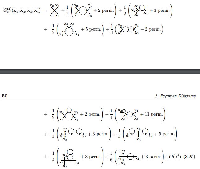
The following resource shows how these rules are used to construct more complex diagrams for higher-order corrections.

Conclusion

In this lesson, we have bridged the gap between the algebraic formalism of Wick's theorem and the intuitive, powerful language of Feynman diagrams. By carrying out a first-order perturbative expansion for the interacting ${\varphi }^4$ theory, we saw how diagrams naturally arise to represent the terms from Wick contractions.

Here are the key takeaways:

• Perturbation theory expands the interacting part of the action, $e^{-S_{int}}$, turning calculations in an interacting theory into sums of Gaussian averages in the free theory.
• The Linked Cluster Theorem ensures that only fully connected diagrams contribute to correlation functions; disconnected vacuum bubbles cancel out.
• Feynman diagrams provide a graphical representation of the terms in the perturbative expansion.
• We established the basic Feynman rules in position space: lines correspond to propagators ($G_0$), vertices to coupling constants ($-u$) and integrations ($\int d^{d}y$), and each diagram has a specific combinatorial symmetry factor.

This lesson concludes our foundational module on Landau-Ginzburg theory and functional integrals. You now have the complete toolset to analyze systems near a critical point using perturbation theory.

In our next module, we will shift our focus to systems with continuous symmetries. We will explore the profound consequences of spontaneous symmetry breaking, leading to the emergence of collective excitations known as Goldstone modes. We will begin by defining spontaneous symmetry breaking and analyzing the mean-field theory of the O(N) model, a generalization of the Ising model that will be central to our future discussions.