Price Visualization with Matplotlib/Plotly

From Data to Chart: Choosing Your Plotting Tool

In Python, there are two dominant libraries for data visualization: Matplotlib and Plotly.

• Matplotlib: The long-standing standard. It's highly versatile and gives you granular control over every aspect of your plot. For financial charts, a library called mplfinance is built on top of it to simplify the process.
• Plotly: A more modern library designed for creating rich, interactive web-based visualizations. Its charts are "live"—you can zoom, pan, and hover over data points to see their values, which is incredibly useful for market analysis.

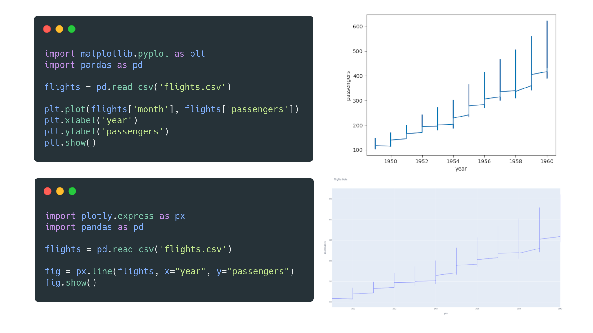
While both are excellent, we will focus on Plotly in this lesson. Its interactive nature closely mimics the experience of professional trading software and is perfect for the kind of deep-dive analysis required for ICT.

A Quick Start: Your First Chart with mplfinance

Before diving into the detailed, layer-by-layer approach of Plotly, let's get a quick win. The mplfinance library makes it incredibly easy to generate a clean candlestick chart with just one line of code. This is great for quick, initial explorations.

First, you'll need to install it. Open your terminal or command prompt and run:
pip install mplfinance

Now, let's assume we have our DataFrame named data from the previous lesson, containing our OHLCV data.

import pandas as pd
import yfinance as yf
import mplfinance as mpf

# Fetch some data to work with (e.g., last 30 days of EUR/USD 4H data)
data = yf.download('EURUSD=X', period='30d', interval='4h')

# That's it! One line to plot the chart.
mpf.plot(data, type='candle', style='yahoo', volume=True)

When you run this, mplfinance automatically identifies the 'Open', 'High', 'Low', 'Close', and 'Volume' columns and produces a static but well-formatted chart. It's a fantastic tool for a fast overview.

Deep Dive: Building an Interactive Chart with Plotly

Now, let's build a fully interactive and customized chart from the ground up using Plotly. This gives you complete control and is the foundation for creating your own bespoke analysis tools.

The following video provides an excellent, comprehensive walkthrough of this process. We will break it down step-by-step, but I encourage you to watch the relevant sections as we go.

Step 1: Setup and Imports

First, we need to import the plotly.graph_objects module, which contains the building blocks for our chart. The conventional alias is go.

import plotly.graph_objects as go
from plotly.subplots import make_subplots

Step 2: Creating the Candlestick Trace

In Plotly, a chart is composed of one or more traces. A trace is a single layer of data visualization, like the candlesticks, a moving average line, or volume bars.

We create a candlestick trace using go.Candlestick. You must tell it which columns from your DataFrame correspond to the open, high, low, and close prices.

# Assuming 'data' is your pandas DataFrame from yfinance

# 1. Create the candlestick trace
candlestick_trace = go.Candlestick(x=data.index,
                                   open=data['Open'],
                                   high=data['High'],
                                   low=data['Low'],
                                   close=data['Close'],
                                   name='Candlesticks')

For a more detailed explanation and code snippet, you can also refer to the "Candlestick Chart" section in the following article.

Step 3: Creating the Figure and Adding Layers

A go.Figure object is the canvas that holds all your traces. We can create a figure and add our candlestick trace to it. To overlay the moving averages we calculated in the last lesson, we add them as go.Scatter traces, which are used for line plots.

Let's put it all together.

# --- First, let's make sure our data has the MAs from the last lesson ---
data['SMA20'] = data['Close'].rolling(window=20).mean()
data['EMA50'] = data['Close'].ewm(span=50, adjust=False).mean()

# 2. Create the Figure object
fig = go.Figure()

# 3. Add the candlestick trace
fig.add_trace(candlestick_trace)

# 4. Add the moving average traces
fig.add_trace(go.Scatter(x=data.index, y=data['SMA20'], 
                         line=dict(color='orange', width=1), name='SMA 20'))
fig.add_trace(go.Scatter(x=data.index, y=data['EMA50'], 
                         line=dict(color='cyan', width=1), name='EMA 50'))

# 5. Display the chart
fig.show()

When you run this code, you'll get your first interactive Plotly chart! You can zoom in on specific areas, pan across the timeline, and see the values of each candle and moving average.

Step 4: Adding Subplots for Volume and Other Indicators

A professional chart often separates price from other indicators like volume or MACD. We can achieve this using make_subplots. This function creates a grid where we can place different traces.

Let's create a chart with two rows: one for price and MAs, and one for volume.

# 1. Create a figure with 2 rows, sharing the x-axis
fig = make_subplots(rows=2, cols=1, shared_xaxes=True, 
                    vertical_spacing=0.05, row_heights=[0.7, 0.3])

# 2. Add price and MAs to the first row (row=1)
fig.add_trace(go.Candlestick(x=data.index, open=data['Open'], high=data['High'],
                            low=data['Low'], close=data['Close'], name='Candles'), 
              row=1, col=1)

fig.add_trace(go.Scatter(x=data.index, y=data['SMA20'],
                         line=dict(color='orange', width=1), name='SMA 20'),
              row=1, col=1)

fig.add_trace(go.Scatter(x=data.index, y=data['EMA50'],
                         line=dict(color='cyan', width=1), name='EMA 50'),
              row=1, col=1)

# 3. Add volume as a bar chart to the second row (row=2)
fig.add_trace(go.Bar(x=data.index, y=data['Volume'], name='Volume', marker_color='lightblue'),
              row=2, col=1)

# 4. Final Touches: Update layout for a clean look
fig.update_layout(title='EUR/USD Interactive Chart',
                  yaxis_title='Price',
                  xaxis_rangeslider_visible=False, # Hide the bulky range slider
                  template='plotly_dark') # Use a dark theme

fig.update_yaxes(title_text="Volume", row=2, col=1)

fig.show()

This code produces a much more organized and professional-looking chart. Notice how we specify row=1, col=1 or row=2, col=1 when adding each trace. The update_layout function is where you can customize titles, colors, and other visual properties. The QuantPy video (sections [7] and [8]) provides an excellent demonstration of these customization options from 13:45 onwards.

# --- First, let's calculate the MACD components ---
ema_12 = data['Close'].ewm(span=12, adjust=False).mean()
ema_26 = data['Close'].ewm(span=26, adjust=False).mean()
data['MACD'] = ema_12 - ema_26
data['Signal_Line'] = data['MACD'].ewm(span=9, adjust=False).mean()

# 1. Create a figure with 3 rows now, and adjust row_heights
fig = make_subplots(rows=3, cols=1, shared_xaxes=True, 
                    vertical_spacing=0.03, row_heights=[0.6, 0.2, 0.2])

# Price and MAs (Row 1 - same as before)
fig.add_trace(go.Candlestick(x=data.index, open=data['Open'], high=data['High'],
                            low=data['Low'], close=data['Close'], name='Candles'), 
              row=1, col=1)
fig.add_trace(go.Scatter(x=data.index, y=data['SMA20'],
                         line=dict(color='orange', width=1), name='SMA 20'),
              row=1, col=1)

# Volume (Row 2 - same as before)
fig.add_trace(go.Bar(x=data.index, y=data['Volume'], name='Volume', marker_color='lightblue'),
              row=2, col=1)

# --- ADDED PART ---
# MACD and Signal Line (Row 3)
fig.add_trace(go.Scatter(x=data.index, y=data['MACD'],
                         line=dict(color='green', width=1), name='MACD Line'),
              row=3, col=1)
fig.add_trace(go.Scatter(x=data.index, y=data['Signal_Line'],
                         line=dict(color='red', width=1), name='Signal Line'),
              row=3, col=1)
# --- END ADDED PART ---

# Update layout
fig.update_layout(title='EUR/USD with Volume and MACD',
                  xaxis_rangeslider_visible=False,
                  template='plotly_dark')

fig.update_yaxes(title_text="Price", row=1, col=1)
fig.update_yaxes(title_text="Volume", row=2, col=1)
fig.update_yaxes(title_text="MACD", row=3, col=1)

fig.show()

Conclusion

Congratulations! You have now mastered a critical skill for any quantitative trader: transforming raw market data into fully interactive, multi-layered charts. This ability to visualize your data and analysis is not just for making pretty pictures; it's fundamental to developing, debugging, and validating your trading ideas.

Key Takeaways:

• Plotly is a powerful Python library for creating interactive financial charts that you can zoom, pan, and inspect.
• Charts are built by adding traces (like go.Candlestick, go.Scatter, go.Bar) to a go.Figure.
• You can create complex layouts with separate panels for price, volume, and indicators using make_subplots.
• The update_layout method allows you to customize titles, colors, templates, and other visual elements to create a professional-looking chart.

Preview for the Next Lesson:
So far in this module, you've learned to fetch, clean, resample, analyze, and visualize market data. You now have a complete toolkit for data handling. In our next module, "Automating Core ICT Concepts," we will begin the most exciting part of your journey. We'll start translating the ICT principles you're familiar with into Python code. Our first objective will be to write a Python function to detect swing highs and swing lows, the absolute bedrock of market structure analysis.