Hello! Let's dive into the practical side of strategy testing.
In our last lesson, we contrasted the two main architectures for backtesting: the realistic but slower event-driven approach and the lightning-fast but less flexible vectorized approach. We concluded that for rapid idea validation and prototyping—essential first steps in developing a trading bot—the speed of vectorized backtesting is a major advantage.
Today, you'll bridge the gap between theory and practice. This lesson fulfills the learning outcome: Build a simple vectorized backtester using pandas for a rule-based strategy. You will write your first Python script that takes historical data, applies a trading rule, and simulates its performance over time. This is a cornerstone skill for your goal of automating ICT strategies.
We won't use a complex ICT rule just yet. Instead, we'll use a simple, classic moving average rule. Why? Because the goal today is to build the engine, not to perfect the car. Once you understand the mechanics of this engine, you can swap out the simple rule for any of your ICT-based rules later.
The Anatomy of a Vectorized Backtest
At its core, a vectorized backtest involves augmenting a price data table with columns that represent our strategy's decisions and performance. The final output often looks something like this:

The process can be broken down into a few key steps:
- Get Data: Load historical price data into a pandas DataFrame.
- Generate Signals: Create a column that indicates when your trading rule is met (e.g.,
TrueorFalse). - Determine Position: Convert the signals into a position state (e.g.,
1for being in a trade,0for being out). This is where we prevent look-ahead bias. - Calculate Returns: Compute the strategy's performance based on the position state.
- Evaluate: Compare the strategy's cumulative returns to a simple "buy and hold" benchmark.
To see this entire workflow in a very simple form, let's start with a short article that demonstrates the core logic.
Backtesting for Beginners: A Simple Start with Python and ...
The article 'Backtesting for Beginners' provides a concise, text-based overview of the entire process using a very basic rule. It's a great way to see the full picture before we dive into a more detailed example.
Please read the sections 'Step 2: Get the Stock Data' through 'Step 5: Visualize the Results'. Focus on understanding the sequence of operations: creating a 'Buy' column, shifting it to create a 'Position' column, and then using that to calculate 'Strategy_Return'.
This article gives you the essential blueprint. Now, let's build a slightly more dynamic version together, using a moving average strategy as our example.
Building the Backtester, Step-by-Step
We'll follow a detailed video tutorial to implement our backtester. It will show you how to calculate a benchmark for comparison and use a real indicator to generate signals.
Step 1: Getting Data and Calculating a Benchmark
Before we test our strategy, we need something to compare it against. The simplest and most common benchmark is "buy and hold." What would our performance have been if we simply bought the asset on day one and held it?
How to Backtest a Trading Strategy in Python (Step-by-Step Beginner Tutorial)
Let's start by loading data and preparing our benchmark. This video, 'How to Backtest a Trading Strategy in Python' by Trading Steady, provides a clear, step-by-step guide. We'll watch the section on downloading data and calculating the benchmark balance.
Watch from 02:04 to 06:50. The first part (until 04:52) covers downloading data with yfinance, which should be a good review. The second part (from 06:00 to 06:50) is key: focus on how the daily returns are calculated and then chained together with .cumprod() to create the bench_bal (benchmark balance) column.
The cumprod() function is short for "cumulative product." It calculates the compounded growth of an initial investment, which gives us our benchmark equity curve.
Step 2: Defining the Rule and Generating Signals
Now for the strategy itself. Our rule will be simple:
Go long when the closing price is above the 200-period moving average. Exit when it falls below.
This is a basic trend-following rule. The video will now show you how to implement this using vectorized operations.
How to Backtest a Trading Strategy in Python (Step-by-Step Beginner Tutorial)
Let's see how to calculate the moving average and create our trading signal. This is where the power of vectorization really shows.
Watch from 12:09 to 14:02. Pay attention to how the .rolling(window=ma).mean() function calculates the moving average for the entire dataset in one line. Then, see how a simple comparison (price['Close'] > price['ma']) creates the boolean long column.
You've just created your raw signal! The long column is True on any day the condition is met and False otherwise.
Step 3: From Signal to Position (Avoiding Look-Ahead Bias)
This is the most important step for ensuring your backtest is valid. We cannot decide to enter a trade and have that trade's profit calculated on the same day. We see a signal at the close of today's candle, so the earliest we can act is at the open of the next candle.
To simulate this, we must shift our signal column forward by one day.
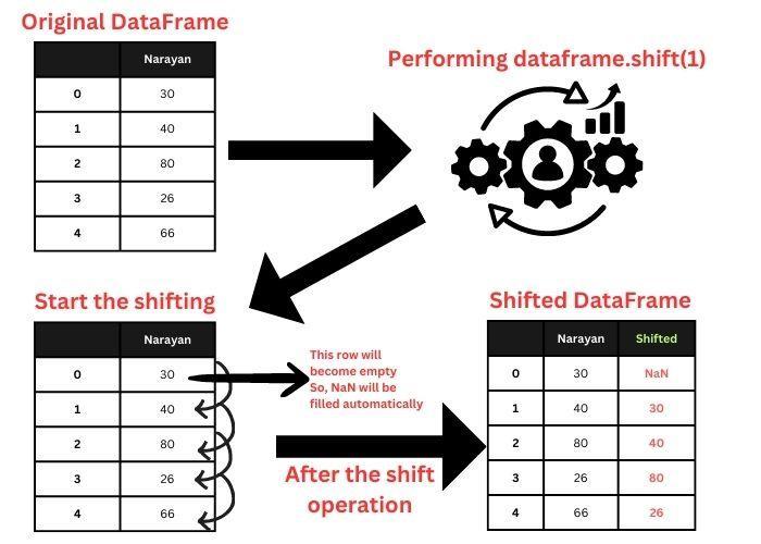
In code, this means our position for today is based on the signal from yesterday. This single operation is how we eliminate look-ahead bias in a vectorized backtest.
Step 4: Calculating Strategy Returns and Comparing Performance
Now that we have a position column that's True (or 1) when we should be in the market and False (or 0) otherwise, we can calculate our strategy's returns.
The logic is simple:
- If our position is
True, our return for the day is the market's return for that day. - If our position is
False, our return for the day is zero (we're in cash).
The video demonstrates a clever way to implement this using numpy.where.
How to Backtest a Trading Strategy in Python (Step-by-Step Beginner Tutorial)
Now let's calculate our strategy's performance and plot everything together.
Watch from 14:52 to 18:00. Notice how the logic uses .shift(1) on the long column to determine the position for the current day. Then, see how np.where is used to calculate the sys_ret (system return). Finally, observe how both the benchmark and system equity curves are plotted on the same chart for direct comparison.
You've now built a complete, simple, vectorized backtester! The final chart gives you instant visual feedback on whether your strategy (in this historical test) was better, worse, or just different from buying and holding.
Test your understanding!
In the video, the moving average period was initially set to 200. The author then changed it to 20 and re-ran the code. Based on your understanding of the code's structure, which line would you modify to test a 50-period moving average instead? After changing it, would you expect the strategy to trade more or less frequently?
Show answer
You would modify the line where the ma variable is defined at the beginning of the script: ma = 200 would become ma = 50.
A 50-period moving average is "faster" or more responsive to recent price changes than a 200-period one. Therefore, the price will cross over it more often. You would expect the strategy to generate more trades (more entries and exits).
Conclusion
Congratulations on building your first backtesting engine! While the moving average rule is basic, the framework you've learned is powerful and reusable. You now know how to translate a trading idea into Python code, test it against historical data, and evaluate its performance—all while respecting the critical rule of avoiding look-ahead bias.
Key Takeaways:
- A vectorized backtest works by adding columns for signals, positions, and returns to a historical price DataFrame.
- Vectorized functions like
.rolling().mean()and.pct_change()perform calculations on the entire dataset at once, making the process extremely fast. - The
.shift(1)function is crucial for preventing look-ahead bias. It ensures your decision to trade is based on information from the previous time step. - Comparing your strategy's equity curve to a benchmark (like buy-and-hold) is essential for evaluating performance.
Preview of the Next Lesson:
Our current backtester gives us a single equity curve. To calculate more advanced metrics like win rate, average profit, or max drawdown, we need a list of individual trades. In the next lesson, we will learn how to generate a series of trades (entry/exit points) from your strategy logic. This will transform our backtester from a high-level performance simulator into a detailed trade analysis tool.