Detecting SMT Divergence

What We're Building: From Chart to Code

Smart Money Technique (SMT) Divergence is a visual pattern. Before we code, let's be crystal clear on what we're asking the computer to find.

• Bearish SMT Divergence: Two positively correlated assets are in an uptrend. Asset A makes a new high, but Asset B fails to do so, creating a lower high. This failure to confirm the strength is a bearish sign.
• Bullish SMT Divergence: The assets are in a downtrend. Asset A makes a new low, but Asset B fails to follow, creating a higher low. This suggests the downward momentum is fading.

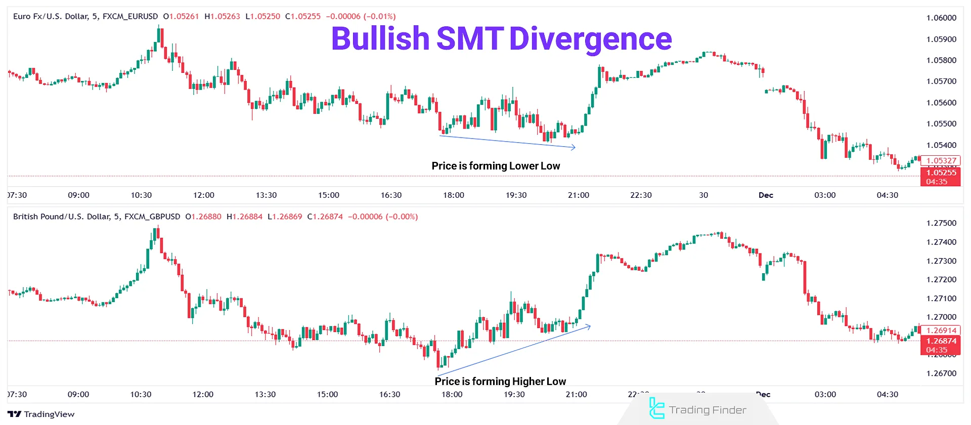
Our task is to translate this visual pattern recognition into a logical, step-by-step algorithm using Python and pandas.

The Algorithmic Logic

At its core, detecting divergence involves three steps:

1. Find the Pivots: We need to programmatically identify the significant swing highs and swing lows in the price data for both assets.
2. Determine the Trend: By comparing consecutive pivots, we can determine if each asset is making higher highs/lower highs or higher lows/lower lows.
3. Compare the Trends: We'll check if the trends of the two assets are moving in opposite directions at the same pivot points. For example, is Asset A making a higher high at the same time Asset B is making a lower high? That's our divergence signal.

Let's implement this step-by-step.

Step 1: Programmatically Identifying Pivot Points

How do we define a swing high or low in code? A common and robust method is to define a pivot as a candle that is higher (for a swing high) or lower (for a swing low) than a certain number of candles on either side of it.

To understand this concept, watch this short clip. The speaker explains how an SMT indicator uses "pivot strength" to define these points.

Now, let's translate that logic into a Python function. The article below provides a well-written function that does exactly this.

Here is the function for easy reference. We will add this to the top of our script.

# Function to identify pivot points
def pivotid(df, l, n1, n2): # n1: bars before, n2: bars after
    if l < n1 or l > len(df) - n2:
        return 0 # Not enough bars to compare, return 0

    pividlow = 1
    pividhigh = 1

    # Check for pivot high
    for i in range(l - n1, l + n2 + 1):
        if(df.High.iloc[l] < df.High.iloc[i]):
            pividhigh = 0
    
    # Check for pivot low
    for i in range(l - n1, l + n2 + 1):
        if(df.Low.iloc[l] > df.Low.iloc[i]):
            pividlow = 0

    if pividhigh and pividlow:
        return 3 # Both a pivot high and low
    elif pividhigh:
        return 2 # Is a pivot high
    elif pividlow:
        return 1 # Is a pivot low
    else:
        return 0 # Not a pivot

Step 2: Determining the Trend Between Pivots

Once we've identified all the pivot points, we need to know the trend. Are the swing highs getting higher or lower? A simple and effective way to do this is to calculate the difference between the current pivot's price and the previous pivot's price.

The pandas.diff() method is perfect for this. When applied to a series of pivot prices, it will return the difference from one pivot to the next.

• A positive result means the new pivot is higher (a higher high or higher low).
• A negative result means the new pivot is lower (a lower high or lower low).

Step 3: Putting It All Together in Code

Let's integrate these steps into the script we started in the last lesson. We will fetch data for two assets, EURUSD=X and GBPUSD=X, and then apply our divergence detection logic.

import yfinance as yf
import pandas as pd
import numpy as np # We need numpy for np.nan

# --- Step 1: Pivot Detection Function ---
def pivotid(df, l, n1, n2):
    if l < n1 or l > len(df) - n2:
        return 0
    
    pividlow = 1
    pividhigh = 1

    for i in range(l - n1, l + n2 + 1):
        if df.High.iloc[l] < df.High.iloc[i]:
            pividhigh = 0
    
    for i in range(l - n1, l + n2 + 1):
        if df.Low.iloc[l] > df.Low.iloc[i]:
            pividlow = 0

    if pividhigh and pividlow:
        return 3
    elif pividhigh:
        return 2
    elif pividlow:
        return 1
    else:
        return 0

# --- Data Fetching and Preparation ---
tickers = ['EURUSD=X', 'GBPUSD=X']
start_date = '2023-10-01'
end_date = '2023-12-31'
data = yf.download(tickers, start=start_date, end=end_date, interval='1h')

# Separate data for each asset
df1 = data.loc[:, (slice(None), tickers[0])].copy()
df1.columns = df1.columns.droplevel(1) # Remove ticker level from columns

df2 = data.loc[:, (slice(None), tickers[1])].copy()
df2.columns = df2.columns.droplevel(1)

# --- Algorithm Implementation for BOTH assets ---
for df in [df1, df2]:
    # 1. Find all pivot points
    # A pivot must be a high/low compared to 10 bars on each side
    df['pivot'] = [pivotid(df, i, 10, 10) for i in range(len(df))]

    # 2. Get the price of the pivots
    df['pivot_high_price'] = np.where(df['pivot'] == 2, df['High'], np.nan)
    df['pivot_low_price'] = np.where(df['pivot'] == 1, df['Low'], np.nan)
    
    # Forward-fill to make comparison easier, then find the trend
    # A positive diff means a higher high/low
    df['trend_high'] = df['pivot_high_price'].ffill().diff()
    df['trend_low'] = df['pivot_low_price'].ffill().diff()

# --- Step 3: Compare Trends to Find Divergence ---
# Merge the dataframes to align the trend data by date
merged_df = pd.merge(df1, df2, on='Date', suffixes=('_1', '_2'))

# Condition for Bullish SMT: Asset 1 makes a lower low, Asset 2 makes a higher low
merged_df['bullish_smt'] = (merged_df['trend_low_1'] < 0) & (merged_df['trend_low_2'] > 0)

# Condition for Bearish SMT: Asset 1 makes a higher high, Asset 2 makes a lower high
merged_df['bearish_smt'] = (merged_df['trend_high_1'] > 0) & (merged_df['trend_high_2'] < 0)

# --- Display Results ---
bullish_divergences = merged_df[merged_df['bullish_smt']]
bearish_divergences = merged_df[merged_df['bearish_smt']]

print(f"--- Found {len(bullish_divergences)} Bullish SMT Signals ---")
print(bullish_divergences[['trend_low_1', 'trend_low_2']])

print(f"\n--- Found {len(bearish_divergences)} Bearish SMT Signals ---")
print(bearish_divergences[['trend_high_1', 'trend_high_2']])

Code Breakdown:

1. Data Separation: We download the data and then create two separate DataFrames, df1 and df2, one for each asset. This makes the logic cleaner.
2. Pivot Identification: We loop through each DataFrame and apply our pivotid function to every row, storing the result (0, 1, 2, or 3) in a new 'pivot' column.
3. Pivot Price & Trend: We create columns to hold the actual price of the pivots. Then we use ffill() (forward fill) to carry the last pivot price forward, and .diff() to calculate the difference from the previous pivot. This gives us our 'trend' columns.
4. Merge & Compare: pd.merge() combines the two DataFrames based on their common 'Date' index. This is crucial as it aligns the trend data perfectly.
5. Divergence Conditions: We create boolean columns (bullish_smt, bearish_smt) that are True only when our SMT conditions are met. For example, for bullish SMT, Asset 1's low trend must be negative (making a lower low) while Asset 2's is positive (making a higher low).
6. Results: Finally, we filter the merged DataFrame to show only the timestamps where a divergence was detected.

Conclusion

Congratulations! You have successfully implemented your first ICT confirmation tool in Python. You've moved beyond simple data fetching and have written an algorithm that can parse price data, identify significant structural points, and detect a nuanced relationship like SMT divergence.

Key Takeaways:

• A complex visual pattern like SMT divergence can be broken down into a logical sequence: find pivots -> determine trend -> compare trends.
• A pivot point can be defined programmatically as an extreme high or low within a specified window of candles.
• The pandas.diff() function is a highly efficient way to calculate the change between consecutive elements, making it ideal for determining the trend between pivots.
• The pandas.merge() function is essential for combining and comparing data from different assets based on a common index like time.

Preview for the Next Lesson:
Detecting SMT divergence provides a powerful confirmation for a potential reversal. The next piece of the puzzle is identifying a high-probability entry point after the divergence has occurred. In our next lesson, we will develop a function to identify an OTE (Optimal Trade Entry) retracement level programmatically. By learning to find the 62%-79% retracement zone, you can begin to combine your SMT confirmation signal with a precise, high-probability entry model.