KV-Cache: Mechanism and Memory in Long-Context Transformers

Introduction

Welcome to the next lesson in our module on Inference at Scale. In our previous discussion, we explored model quantization as a powerful technique for reducing the memory footprint and accelerating computation by using lower-precision data types. We saw that this helps alleviate the memory bandwidth bottleneck, which is often the primary limiter of LLM inference performance.

Today, we're going to dive into another, equally critical aspect of the memory puzzle in Transformer inference: the Key-Value (KV) cache. While quantization shrinks the model's static weights, the KV cache represents a dynamic memory consumer that grows with every token generated. For long-context models, its memory consumption can dwarf that of the model weights themselves.

This lesson will address the learning outcome: Describe the KV-cache mechanism in Transformer inference and its memory implications for long-context models. We will explore why this cache is necessary, how it works, and precisely how it becomes a dominant factor in the system design and performance of LLM inference servers.

The Problem: The Inefficiency of Autoregressive Generation

To understand the need for the KV cache, we first need to revisit how decoder-only Transformers, like the GPT family, generate text. They operate autoregressively, meaning they produce one token at a time, with each new token conditioned on all the tokens that came before it.

This process relies on the self-attention mechanism. At each step, the model must calculate how the current token "attends" to all previous tokens in the sequence to gather the necessary context for predicting the next token.

Without any optimization, this is incredibly inefficient. To generate the 100th token, the model would perform attention over the preceding 99 tokens. To generate the 101st token, it would have to repeat the entire process, performing attention over all 100 preceding tokens. This redundant recalculation of attention for tokens that have already been processed results in computational complexity that scales quadratically with the sequence length ($O(n^2)$). For long sequences, this is computationally prohibitive.

To get a clearer picture of how information is processed in the attention mechanism, the following video provides an excellent visual and mathematical breakdown.

As the video illustrates, the Key and Value matrices contain information derived from all tokens in the current context. The core inefficiency is that for a standard autoregressive loop, these K and V matrices for the initial tokens would be recomputed at every single step.

The Solution: The Key-Value (KV) Cache

The KV cache is the fundamental optimization that solves this quadratic scaling problem by introducing statefulness into the generation process. The core idea is simple: if the Key and Value vectors for previous tokens don't change, don't recompute them. Instead, store them.

The inference process is thus split into two distinct phases:

1. Prefill (or Processing the Input):

   • When the model receives an initial prompt, it processes all of its tokens in a single, highly parallel forward pass.
   • During this pass, it calculates the Key and Value vectors for every token in the prompt, across all attention heads and all layers.
   • These computed K and V tensors are then stored in dedicated memory on the GPU. This is the "prefilled" KV cache.
   • This phase is typically compute-bound because it involves large matrix-matrix multiplications that can saturate the GPU's computational units.

2. Decode (or Generating the Output):

   • To generate each new token, the model only needs to process the single most recent token through its layers.
   • For this new token, it computes a new Query vector and a new K/V pair.
   • The new Query vector then attends to the Keys of all previous tokens, which are quickly retrieved from the KV cache, plus the newly computed Key.
   • The resulting attention scores are used to create a weighted sum of the Values from the KV cache and the new Value.
   • Finally, the new K/V pair is appended to the cache for the next step.
   • This phase is typically memory-bandwidth-bound, as the main operation is moving the large KV cache tensors from GPU memory (HBM) to the on-chip SRAM for computation.

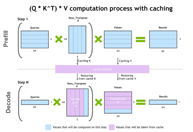
The following video provides a clear explanation of this mechanism, showing how it avoids redundant work.

By caching the K and V tensors, the computational cost per generated token becomes linear ($O(n)$) instead of quadratic, making real-time generation for long sequences feasible. However, this elegant solution introduces a new, significant challenge.

The New Problem: The Memory Footprint of the KV Cache

We've traded a compute problem for a memory problem. The KV cache must store two tensors (K and V) for every single token in the sequence, for every attention head, for every layer in the model. As the context grows, so does the cache, consuming a massive amount of GPU VRAM.

The size of the KV cache can be calculated with the following formula:

Total KV Cache Size (in bytes) = batch_size × sequence_length × num_layers × hidden_size × 2 × precision_in_bytes

Where:

• hidden_size is the dimension of the model's hidden state, which is equivalent to num_heads × head_dimension.
• The factor of 2 accounts for storing both the Key and Value tensors.
• precision_in_bytes is the number of bytes per value (e.g., 2 for FP16/BF16, 1 for INT8).

Let's ground this with a concrete example.

As the article demonstrates, for a 7B parameter model like Llama 2 7B, the model weights in FP16 take up ~14 GB. With a batch size of 1 and a sequence length of 4096, the KV cache alone consumes ~2 GB. If you increase the batch size to 32, the KV cache balloons to ~64 GB, far exceeding the memory required for the model weights.

This has profound implications for system design:

• Dominant Memory Consumer: For long-context or high-throughput (large batch) scenarios, the KV cache, not the model weights, becomes the primary consumer of GPU memory.
• Memory-Bandwidth Bottleneck: The performance of the decode phase is no longer limited by how fast the GPU can do math, but by how fast it can read the massive KV cache from HBM into the SMs for each new token.
• Limited Context/Batch Size: The total available VRAM on a GPU places a hard limit on the maximum sequence length and batch size that can be served.

The following video provides another excellent calculation that reinforces this point.

Mitigating the Memory Burden

The enormous size of the KV cache has spurred significant innovation in model architecture and inference systems. While a deep dive into these solutions is for future lessons, it's important to be aware of the main strategies.

1. Architectural Changes: MQA and GQA

One way to reduce the cache size is to change the model's attention mechanism itself.

• Multi-Query Attention (MQA): Instead of each attention head having its own K and V projections, all heads within a layer share a single set of K and V tensors. This drastically reduces the size of the KV cache (by a factor equal to the number of heads) but can lead to a drop in model quality.
• Grouped-Query Attention (GQA): A compromise between standard multi-head attention (MHA) and MQA. Heads are divided into groups, and heads within each group share K and V tensors. This provides a balance, reducing memory usage significantly while retaining most of the model quality. Models like Llama 2/3 use GQA.

2. Efficient Memory Management: PagedAttention

Another approach is not to change the cache's size, but to manage its memory allocation more intelligently. Systems often pre-allocate a contiguous block of memory for the KV cache to accommodate the maximum possible sequence length. This is wasteful, as most sequences are much shorter.

PagedAttention, an algorithm popularized by the vLLM library, takes inspiration from virtual memory and paging in operating systems. It partitions the KV cache into non-contiguous blocks ("pages"). Memory is allocated on-demand as generation proceeds, eliminating internal fragmentation and overallocating memory. This allows the system to pack more requests into a batch, significantly increasing throughput.

Conclusion

In this lesson, we dissected the KV cache, a cornerstone optimization for Transformer inference. While it elegantly solves the quadratic complexity of autoregressive generation, it introduces a new, formidable challenge in the form of massive memory consumption.

Key Takeaways:

• Mechanism: The KV cache stores the Key and Value tensors from the self-attention layers for all processed tokens, avoiding redundant computation and changing the per-token generation complexity from quadratic to linear.
• Two Phases: Inference operates in a compute-bound prefill phase (processing the prompt) and a memory-bandwidth-bound decode phase (generating new tokens). The KV cache is populated in the first and utilized in the second.
• Memory Implications: The cache size scales linearly with sequence length and batch size. For long-context models, it is often the largest consumer of GPU VRAM, making inference a memory-bandwidth-bound problem.
• Trade-off: The KV cache is a classic example of a space-time trade-off. We trade significantly more memory (space) for a dramatic reduction in computation time.

Preview of the Next Lesson:

Understanding the KV cache and its memory management challenges is the perfect foundation for our next topic. We will explore specialized serving libraries like vLLM and TensorRT-LLM, which are designed specifically to tackle these issues. We will see how they implement advanced techniques like PagedAttention to dramatically improve memory efficiency and unlock higher throughput for LLM inference at scale.