Virtual vs. Non-Virtual Calls: A Runtime Performance Comparison

1. The Anatomy of a Virtual Function Call

Let's start with a classic polymorphic scenario:

// Base class with virtual functions
struct Animal {
    virtual void speak() { /* ... */ }
};

// Derived class overriding the virtual function
struct Dog : public Animal {
    void speak() override { /* ... */ }
};

int main() {
    Animal* p_animal = new Dog(); // Base pointer, Derived object
    p_animal->speak();            // Which speak() gets called?
    delete p_animal;
}

The call p_animal->speak() is where dynamic dispatch happens. At compile time, the compiler only knows that p_animal is an Animal*. It cannot hardcode a jump to Animal::speak or Dog::speak. Instead, it generates code to perform a lookup at runtime.

This lookup follows a precise sequence of steps:

1. Get the object address: The process starts with the address stored in p_animal.
2. Find the vptr: The code dereferences p_animal to access the Dog object's memory. It reads the first 8 bytes (on a 64-bit system), which is the hidden vptr.
3. Find the vtable: The vptr's value is the memory address of the Dog class's vtable. The code follows this pointer to the vtable, which is located in a read-only segment of the program.
4. Find the function address: The compiler knows that speak() is the first virtual function in the Animal class, so its entry is at index 0 of the vtable. The code reads the function pointer from this slot. In this case, because the object is a Dog, it gets the address of Dog::speak.
5. Call the function: The CPU executes a call instruction using the address retrieved in the previous step.

To see this process visualized clearly, watch the following short segment.

The diagram below, based on the article we'll review next, shows this entire chain from the object on the stack to the function code in the text section.

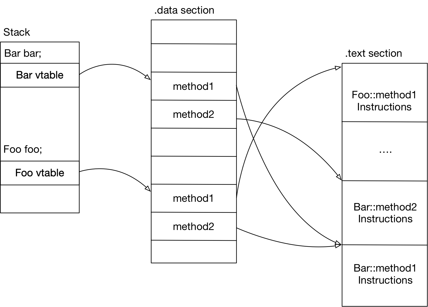
2. From C++ to Assembly: The Ground Truth

Your desire to understand things from first principles is best satisfied by looking at the assembly code the compiler generates. This is as close as we can get to what the CPU actually executes. Given your background in C, you'll recognize that the "magic" of a virtual call is just a series of pointer dereferences.

The following article demonstrates this by examining the assembly for a virtual call inside a loop.

Let's dissect the core instructions for ptr->method1() from that article:

// Let's assume the current object pointer `ptr` is in register `r10` for clarity.

// 1. Get the vptr from the object.
//    Load the value at the address in r10 into r11. This is the vptr.
mov r11, QWORD PTR [r10]

// 2. Get the function address from the vtable.
//    Load the value at the address in r11 (the vtable's start) into r12.
//    This is the address of the first virtual function (method1).
mov r12, QWORD PTR [r11] 

// 3. Call the function.
//    Pass the 'this' pointer (the object's address) in the first argument register (rdi on Linux).
mov rdi, r10
//    Execute an indirect call to the address held in r12.
call r12

Compare this to a non-virtual call (call MyClass::my_function), which is a single instruction that jumps to a hardcoded address known at compile time. The virtual call involves extra memory reads and an indirect jump, which brings us to the question of performance.

3. The Performance Cost of Dynamic Dispatch

A virtual function call has overhead from three primary sources.

A. Direct Cost: Indirection and Cache Misses

The most obvious cost is the pointer chasing we just saw: Object -> vptr -> vtable -> Function. Each of these arrows represents a memory access. In a worst-case scenario where the object, the vtable, and the function code are not in the CPU cache, each step could trigger a slow trip to main memory.

However, as the following video explains, this direct cost is often small for well-behaved programs where the data is hot in the cache.

B. Indirect Cost: The Inlining Barrier

The most significant performance penalty of virtual calls is often indirect: they prevent compiler optimizations, most notably inlining.

• Inlining is when the compiler replaces a function call with the body of the function itself, eliminating the overhead of setting up a stack frame and jumping. More importantly, it exposes the function's code to the surrounding context, enabling a cascade of further optimizations (like vectorization or removing redundant checks).
• With a virtual call, the compiler doesn't know the destination at compile time, so it cannot inline the function. It must generate a full, heavyweight function call.

This video segment explains this crucial concept beautifully.

C. CPU Cost: Branch Misprediction

Modern CPUs use speculative execution to improve performance. For an indirect jump like a virtual call, the CPU's branch predictor tries to guess the destination address.

• If you are looping through a collection of objects that are all of the same type (e.g., a std::vector of Dog objects), the branch predictor will quickly learn the destination and the overhead becomes minimal.
• If the types are random, the predictor will constantly guess wrong. A misprediction is expensive, as the CPU must discard the speculatively executed work and restart the pipeline from the correct location.

This CppCon talk provides a powerful experiment demonstrating this effect.

4. Compiler Magic: Devirtualization

Given these costs, you might think virtual functions are a performance landmine. However, modern compilers are incredibly smart and can often eliminate the overhead through an optimization called devirtualization. The compiler tries to prove the concrete type of an object at a call site. If it succeeds, it can replace the virtual call with a direct, inlinable call.

Conclusion

Today, we traced the entire lifecycle of a virtual function call, from high-level C++ down to the assembly instructions. We've seen that it's a deterministic, mechanical process, not magic.

Key Takeaways:

• A virtual call is resolved at runtime through a two-step pointer lookup: object -> vptr -> vtable -> function_address.
• The primary performance cost of virtual functions is not the direct lookup overhead, but the indirect cost of blocking compiler optimizations, especially inlining.
• CPU-level features like branch prediction significantly affect performance; predictable call patterns are fast, while random patterns are slow due to mispredictions.
• Modern compilers are highly adept at devirtualization, often succeeding in converting virtual calls back into faster, direct calls when the object's type can be determined.

In our next lesson, we will address a critical and common bug in polymorphic code: resource leaks. We will learn why you must implement and explain the necessity of virtual destructors for preventing resource leaks in polymorphic deletion. This is a direct application of the virtual mechanism we've just studied to ensure program correctness.