Introduction
In the past few lessons, you've done the important work of converting the probability functions for the Binomial, Poisson, Normal, Gamma, and Negative Binomial distributions into the standard exponential family form. This gave you a foundational understanding of their mathematical structure and the origin of their key components like and .
Now, we shift from derivation to application. In your exam, you'll likely face questions that describe a scenario and ask you to choose the correct statistical approach. A critical first step is selecting the right probability distribution for the outcome variable. This lesson is designed to equip you with a clear, systematic process for making that choice.
By the end of this lesson, you will be able to analyze a data description or a set of descriptive statistics and confidently select the most appropriate exponential family distribution for modeling the response variable.
A Framework for Choosing Your Distribution
To select the right distribution, you need to be a detective and look for clues about your response variable, which we'll call . Almost always, the choice comes down to answering three key questions:
- What is the nature of the data? Is it discrete (e.g., counts) or continuous (e.g., measurements)?
- What are its boundaries? Is the data unbounded, does it have a lower bound (like 0), or is it bounded on both ends (like a proportion between 0 and 1)?
- What is the relationship between its mean and variance? Is the variance constant, equal to the mean, or does it increase with the mean in a specific way?
The following resource provides an excellent decision chart that visualizes this process.
The book 'New statistics for design researchers' offers a practical guide to GLMs. We'll start with its decision chart, which provides a great roadmap for selecting a distribution.
In this resource, find and study 'Figure 7.1: Decision chart for Generalized Linear Models'. Pay close attention to the questions at each branching point of the chart. Notice how asking about the nature of the data (discrete vs. continuous) and its boundaries helps narrow down the choices.
Let's break down the branches of this decision tree.
1. Discrete (Count) Data
When your response variable consists of counts, you have three primary options. The choice among them often depends on the data's boundaries and its mean-variance relationship.

Binomial Distribution
- Use when: Your data represents the number of "successes" in a fixed number of trials ().
- Boundaries: Bounded below by 0 and above by a known integer .
- Special Case (Binary Data): A very common case is when . The outcome is one of two possibilities (e.g., yes/no, success/failure, 0/1). This is often called Logistic Regression.
- Mean-Variance: . The variance depends on the mean.
- Example: Modeling the number of tasks a user completes correctly out of 10 total tasks. Here, .
Poisson Distribution
- Use when: Your data represents counts of events occurring in a fixed interval of time or space, with no specific upper limit.
- Boundaries: Bounded below by 0, but theoretically unbounded above.
- Mean-Variance: The key assumption is that the mean equals the variance, i.e., .
- Example: Modeling the number of clicks on a webpage per minute.
Negative Binomial (NB2) Distribution
- Use when: Your data represents counts (like Poisson), but the variance is clearly larger than the mean. This situation is called overdispersion. In practice, real-world count data is often overdispersed, making the Negative Binomial a very useful alternative to Poisson.
- Boundaries: Same as Poisson (0 to infinity).
- Mean-Variance: . Specifically for the NB2 model, the variance function is , where is the dispersion parameter.
- Example: Modeling the number of articles a student writes in a semester. Most students write a few, but a few prolific students write many, increasing the variance beyond what a Poisson model would predict.
2. Continuous Data
When your response variable can take any value within a range, it's continuous. The choice of distribution depends on the data's boundaries and its shape (symmetric vs. skewed).
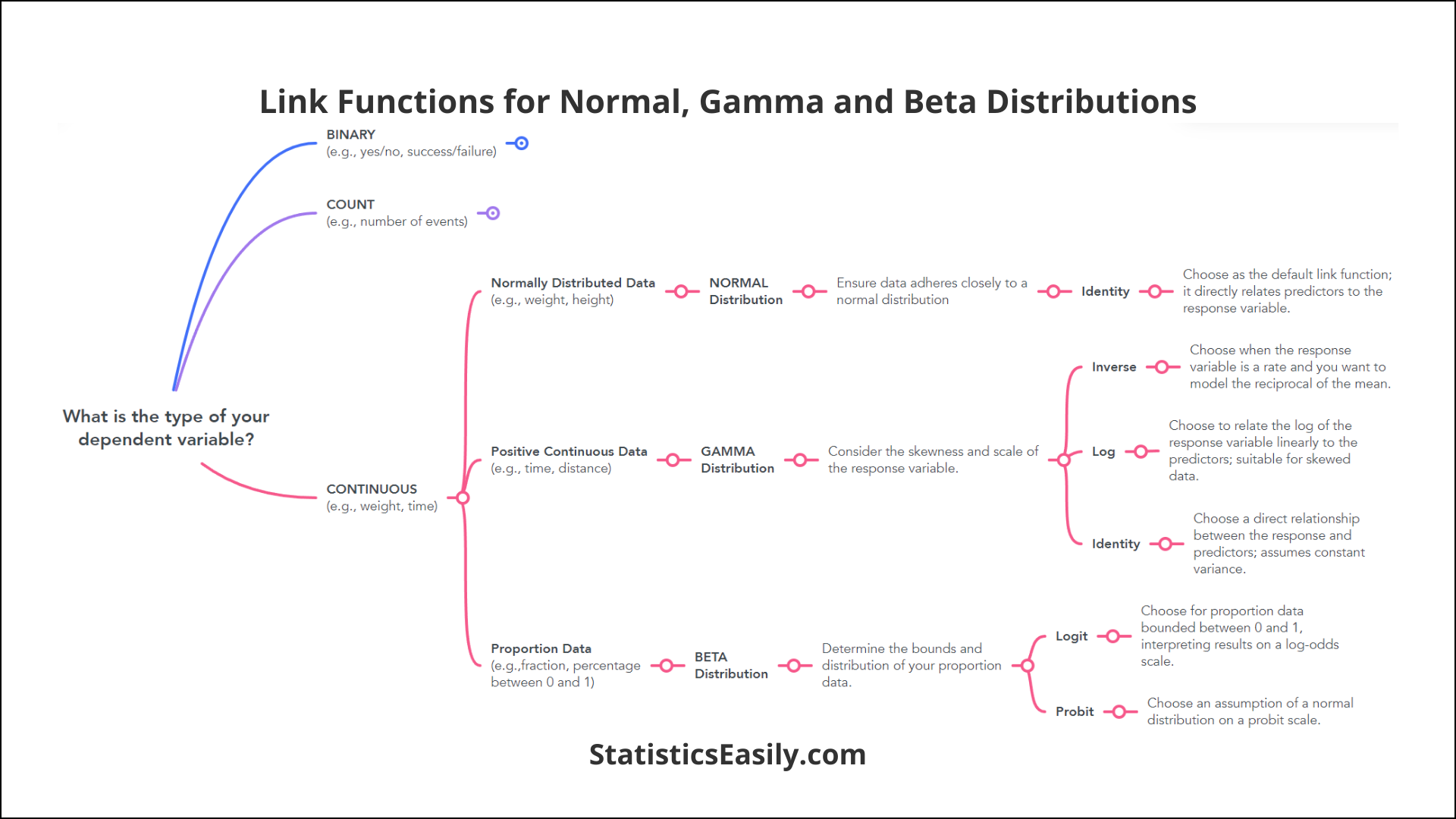
Normal (Gaussian) Distribution
- Use when: The data is continuous, roughly symmetric (bell-shaped), and theoretically unbounded.
- Boundaries: Unbounded (-, +). It can be a reasonable approximation if the actual boundaries are very far from the data's mean.
- Mean-Variance: The mean and variance are independent parameters. The variance is assumed to be constant.
- Example: Modeling adult human heights.
Gamma Distribution
- Use when: The data is continuous, strictly positive, and skewed to the right.
- Boundaries: Bounded below by 0, unbounded above.
- Mean-Variance: The variance is proportional to the mean squared: . This means the standard deviation grows proportionally with the mean.
- Example: Modeling the time to failure of a mechanical part or the amount of an insurance claim.
Beta Distribution
- Use when: The data is continuous and represents a proportion, percentage, or rate.
- Boundaries: Bounded on both ends, between 0 and 1. (Note: Standard Beta regression requires values to be strictly between 0 and 1, so values of exactly 0 or 1 may need a slight adjustment).
- Example: Modeling the proportion of a student's budget spent on textbooks.
The Decisive Role of the Mean-Variance Relationship
As you've seen, the relationship between the mean and variance is a powerful clue. This isn't just a practical trick; it's a deep property of the exponential family. A key theoretical result states that the variance function, which describes how the variance depends on the mean, uniquely identifies the distribution.
A Primer on the Exponential Family of Distributions
To understand the theory behind using the mean-variance relationship, let's consult 'A Primer on the Exponential Family of Distributions'. This will solidify why this is such a reliable decision rule.
First, read the section 'The Variance Function Var(Y) and Uniqueness' (page 122). Focus on the 'Uniqueness Property'. Then, review the summary table of variances under the 'Moments' heading on page 131. This table directly links each distribution to its variance function.
Here is a summary of the variance functions for the key distributions, where and is the dispersion parameter.
| Distribution | Variance Function | Key Implication |
|---|---|---|
| Normal | Variance is constant (). | |
| Poisson | Variance equals the mean. | |
| Binomial | Variance is a quadratic function of the mean. | |
| Gamma | Standard deviation is proportional to the mean. | |
| Negative Binomial | Variance is greater than the mean. | |
| Inverse Gaussian | Variance grows rapidly with the mean. |
This table is a powerful tool for your exam. If a problem gives you the mean and variance, or describes how you expect the variance to behave, you can use this table to make a strong, defensible choice.
Practice Scenarios
Let's apply this framework. For each scenario, decide on the most appropriate distribution for the response variable.
Scenario 1:
You are analyzing data on the number of non-conformities in batches of a manufactured product. The mean number of non-conformities per batch is 4.2, and the variance is 9.5.
Solution
* **Nature:** The data is a count (number of non-conformities), so it's discrete. * **Boundaries:** It is bounded below by 0. * **Mean-Variance:** The variance (9.5) is significantly greater than the mean (4.2). This is a classic case of overdispersion. * **Conclusion:** The **Negative Binomial** distribution is the most appropriate choice.Scenario 2:
A political scientist is modeling the outcome of an election in different districts. The response variable is the proportion of votes received by a particular candidate in each district.
Solution
* **Nature:** The data is a proportion, so it's continuous. * **Boundaries:** It is naturally bounded between 0.0 and 1.0. * **Conclusion:** The **Beta** distribution is the correct choice for modeling proportions.Scenario 3:
An e-commerce company runs an A/B test on a new "Buy Now" button. For each of the 10,000 users who visit the page, the company records whether the user clicked the button (1) or not (0).
Solution
* **Nature:** The data for each user is binary (0 or 1), which is a form of discrete data. * **Boundaries:** The outcome for each trial is either 0 or 1. * **Conclusion:** This is a classic binary outcome, which is modeled using a **Binomial** distribution with $n=1$ (also known as a Bernoulli distribution). This is the basis for logistic regression.Scenario 4:
A call center wants to model the duration (in minutes) of support calls. A histogram of the call durations shows that most calls are short, but there is a long tail of very long calls. The data is continuous and cannot be negative.
Solution
* **Nature:** The data is continuous. * **Boundaries:** It is bounded below by 0. * **Shape:** The description of a long tail to the right indicates the data is right-skewed. * **Conclusion:** The **Gamma** distribution is a suitable choice for right-skewed, strictly positive continuous data. (An Exponential distribution could also be a candidate, but Gamma is more flexible).Conclusion
You have now learned a systematic process for selecting the appropriate distribution from the exponential family—a critical skill for both theoretical understanding and practical application in your exam.
Key Takeaways:
- Your starting point is the response variable. Analyze its characteristics.
- Ask the three key questions: Is it discrete or continuous? What are its boundaries? What is the relationship between its mean and variance?
- Use the Mean-Variance relationship as your power tool. The uniqueness property of the exponential family means the variance function is a reliable guide to the underlying distribution.
In the previous lessons, you learned how to derive the mathematical forms of these distributions. Now you know how to choose among them. The next step is to learn how to fit these models to data. In the next module, we will dive into parameter estimation, exploring how algorithms like Fisher Scoring and Iteratively Reweighted Least Squares (IRWLS) are used to find the best-fitting coefficients for a GLM.