Deriving Score Equations from Log-Likelihood

Introduction

Welcome back! In our previous lesson, we established the foundation for parameter estimation in Generalized Linear Models (GLMs) by learning how to formulate the log-likelihood function, $l (β)$ . This function tells us how "plausible" a given set of model coefficients $β$ is, based on our observed data.

Our ultimate goal is to find the coefficients $β^$ that maximize this function. From basic calculus, you know that to find the maximum of a function, you take its derivative, set it to zero, and solve. That's exactly what we're going to do today.

This lesson will focus on deriving the score equations, which are the set of equations obtained by differentiating the log-likelihood function with respect to each model parameter and setting the result to zero. Mastering this step is crucial as it forms the basis of the numerical algorithms used to fit GLMs.

The Score Function and Score Equations

The process of finding the maximum likelihood estimates (MLEs) involves these key steps:

Formulate the log-likelihood function, $l (β)$ . (You learned this last lesson).
Differentiate $l (β)$ with respect to each parameter $β_{j}$ to get the score function.
Set these derivatives to zero to form the score equations.
Solve the score equations for $β$ .

Let's formalize the definition of the score function.

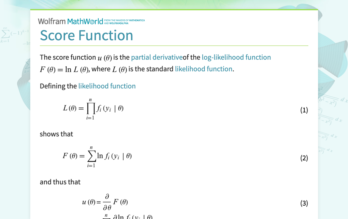
Score Function Definition and Derivation — This image from Wolfram MathWorld shows the definition of the score function, denoted $u(\theta)$, as the partial derivative of the log-likelihood function with respect to the parameter $\theta$. For a model with multiple parameters $\boldsymbol{\beta} = (\beta_0, \beta_1, \ldots, \beta_p)$, the score function is a vector of these partial derivatives.

The score function, denoted $U (β)$ , is the vector of these partial derivatives:

U (β) = \frac{\partial l ( β )}{\partial β} = \frac{\partial l ( β )}{\partial β _{0}} \frac{\partial l ( β )}{\partial β _{1}} ⋮ \frac{\partial l ( β )}{\partial β _{p}}

The score equations are the system of equations we need to solve, which is simply the score function set to a vector of zeros:

U (β^) = 0

The solution, $β^$ , is our Maximum Likelihood Estimate.

Deriving the Score Equations: The General Case

While we can differentiate the log-likelihood for each specific distribution, it's more powerful to derive a general formula that works for any GLM in the exponential family. This requires the chain rule.

Recall the log-likelihood for a single observation $i$ :

l_{i} = \frac{y _{i} θ _{i} - b ( θ _{i} )}{ϕ} + c (y_{i}, ϕ)

We need to find $\frac{\partial l _{i}}{\partial β _{j}}$ . The parameters $β$ are linked to $θ_{i}$ through the linear predictor and link function. Here is the chain of dependencies:

β_{j} \to η_{i} = x_{i}^{T} β \to μ_{i} = g^{- 1} (η_{i}) \to θ_{i}

By the chain rule, the derivative is:

\frac{\partial l _{i}}{\partial β _{j}} = \frac{\partial l _{i}}{\partial θ _{i}} \cdot \frac{\partial θ _{i}}{\partial μ _{i}} \cdot \frac{\partial μ _{i}}{\partial η _{i}} \cdot \frac{\partial η _{i}}{\partial β _{j}}

Let's find each component. The following resource provides the mathematical details for this derivation.

[PDF] MATH 523 - Generalized Linear Models - Léo Belzile, PhD

These notes from Léo Belzile's course on GLMs provide a concise derivation of the general form of the score equations. We'll focus on the section that assembles the chain rule.

Please read the short section 'Iteratively reweighted least-squares' on page 28, specifically focusing on the derivation steps near the bottom of the page that start with 'By the chain rule, ∂ℓ(y; θ, φ)/∂βj = ...' and the three key identities: dµ/dθ = V(µ), ∂η/∂βj = xj, and the one relating ∂ℓ/∂θ to (y-µ).

As shown in the resource, the components of the chain rule are:

$\frac{\partial l _{i}}{\partial θ _{i}} = \frac{y _{i} - b ^{'} ( θ _{i} )}{ϕ} = \frac{y _{i} - μ _{i}}{ϕ}$
$\frac{\partial θ _{i}}{\partial μ _{i}} = \frac{1}{d μ _{i} / d θ _{i}} = \frac{1}{V ( μ _{i} )}$ (since $Var (Y_{i}) = ϕ V (μ_{i})$ )
$\frac{\partial μ _{i}}{\partial η _{i}} = \frac{1}{g ^{'} ( μ _{i} )}$
$\frac{\partial η _{i}}{\partial β _{j}} = x_{ij}$

Putting it all together for one observation:

\frac{\partial l _{i}}{\partial β _{j}} = (\frac{y _{i} - μ _{i}}{ϕ}) (\frac{1}{V ( μ _{i} )}) (\frac{1}{g ^{'} ( μ _{i} )}) x_{ij}

The full score equation for parameter $β_{j}$ is the sum over all $n$ observations, set to zero:

U_{j} (β) = i = 1 \sum n \frac{( y _{i} - μ _{i} ) x _{ij}}{ϕ V ( μ _{i} ) g ^{'} ( μ _{i} )} = 0

A Major Simplification: Canonical Links

This formula simplifies beautifully when we use a canonical link function. For a canonical link, $θ_{i} = η_{i}$ . The chain rule becomes much shorter, as $μ_{i}$ is no longer an intermediate step between $θ_{i}$ and $η_{i}$ . The derivative is simply:

\frac{\partial l _{i}}{\partial β _{j}} = \frac{\partial l _{i}}{\partial θ _{i}} \cdot \frac{\partial θ _{i}}{\partial β _{j}} = (\frac{y _{i} - μ _{i}}{ϕ}) x_{ij}

The score equation for $β_{j}$ with a canonical link is:

U_{j} (β) = i = 1 \sum n \frac{( y _{i} - μ _{i} ) x _{ij}}{ϕ} = 0

Since $ϕ$ is a constant, we can ignore it for finding the root, giving the elegantly simple form:

i = 1 \sum n (y_{i} - μ_{i}) x_{ij} = 0

This means the MLE is found at the point where the model's residuals, $y_{i} - μ_{i}$ , are orthogonal to (uncorrelated with) the predictor variables $x_{ij}$ . This is a direct generalization of the principle behind ordinary least squares regression.

Worked Example: Poisson Regression

Let's apply this to the Poisson GLM, which uses a canonical log link. In the previous lesson, we found its log-likelihood:

l (β) = i = 1 \sum n (y_{i} (x_{i}^{T} β) - exp (x_{i}^{T} β) - lo g (y_{i}!))

We can derive the score equations by direct differentiation. Let's see this in action.

[PDF] MATH 523 - Generalized Linear Models - Léo Belzile, PhD

Let's read the section 'Example 2.9 (Poisson regression)' in the MATH 523 notes. It shows the step-by-step differentiation of the Poisson log-likelihood.

Read 'Example 2.9 (Poisson regression)' on page 32. Follow how the partial derivative ∂ℓn(β)/∂βj is taken, leading to the final expression \sum_{i=1}^{n} x_{ij}(y_i - \mu_i).

As the resource demonstrates, differentiating $l (β)$ with respect to a single parameter $β_{j}$ gives:

\frac{\partial l}{\partial β _{j}} = i = 1 \sum n (y_{i} x_{ij} - exp (x_{i}^{T} β) \cdot x_{ij})

Since for a Poisson model with a log link, $μ_{i} = exp (x_{i}^{T} β)$ , we can rewrite this as:

\frac{\partial l}{\partial β _{j}} = i = 1 \sum n (y_{i} x_{ij} - μ_{i} x_{ij}) = i = 1 \sum n x_{ij} (y_{i} - μ_{i})

Setting this to zero gives the score equation for $β_{j}$ :

i = 1 \sum n x_{ij} (y_{i} - μ_{i}) = 0

This exactly matches the simplified formula for canonical links, since for the Poisson distribution, $ϕ = 1$ .

Worked Example: Logistic Regression

Now let's do the same for logistic regression, which uses a Binomial distribution and the canonical logit link. The log-likelihood is:

l (β) = i = 1 \sum n [y_{i} (x_{i}^{T} β) - lo g (1 + exp (x_{i}^{T} β))]

Let's see the derivation for its score equations.

[PDF] MATH 523 - Generalized Linear Models - Léo Belzile, PhD

The MATH 523 notes also have a very clear derivation for the logistic regression score equations. It's nearly identical to the Poisson case.

Please read the section '4.1 Binomial Model and Logistic Regression' on page 62. Focus on the final two equations, where ∂ℓn(β)/∂β is derived.

Differentiating with respect to $β_{j}$ involves the chain rule for the second term:

\frac{\partial}{\partial β _{j}} lo g (1 + exp (x_{i}^{T} β)) = \frac{1}{1 + exp ( x _{i}^{T} β )} \cdot exp (x_{i}^{T} β) \cdot x_{ij}

The fraction is the inverse logit function, which is exactly the mean $μ_{i}$ (often written as $π_{i}$ for probabilities). So the derivative is simply $μ_{i} x_{ij}$ .

Combining terms, the derivative of the log-likelihood is:

\frac{\partial l}{\partial β _{j}} = i = 1 \sum n (y_{i} x_{ij} - μ_{i} x_{ij}) = i = 1 \sum n x_{ij} (y_{i} - μ_{i})

Again, this perfectly matches our general formula for a canonical link, giving us the score equation:

i = 1 \sum n x_{ij} (y_{i} - μ_{i}) = 0

Conclusion

In this lesson, you have moved from constructing the log-likelihood function to deriving the equations needed to optimize it. This is the heart of the estimation process.

Key Takeaways:

The score function is the vector of first partial derivatives of the log-likelihood function with respect to the model parameters $β$ .
The score equations are formed by setting the score function to zero. Solving them yields the Maximum Likelihood Estimates.
We derived a general formula for the score equations using the chain rule, which applies to any GLM.
For canonical links, this formula simplifies to the intuitive expression $\sum (y_{i} - μ_{i}) x_{ij} = 0$ , meaning the model residuals are uncorrelated with the predictors.
We confirmed this result by directly differentiating the log-likelihood for Poisson and logistic regression.

You now have the equations, but how do you solve them? Except for the simplest cases, these are non-linear equations with no closed-form solution. They must be solved numerically. In our next lesson, we will explore the main algorithm used for this purpose: Fisher scoring, and see how it is implemented as Iteratively Reweighted Least Squares (IRWLS).

Recommended resources

Introduction

The Score Function and Score Equations

Deriving the Score Equations: The General Case

A Major Simplification: Canonical Links

Worked Example: Poisson Regression

Worked Example: Logistic Regression

Conclusion