Bias-Variance Tradeoff Explained

An Intuitive Picture: Bias and Variance

Before diving into the mathematics, let's build an intuition for what bias and variance represent.

• Bias is a measure of a model's systematic error. A high-bias model makes strong assumptions about the data (e.g., assuming a linear relationship where it's actually quadratic). This leads it to consistently miss the true signal, regardless of the specific training data it sees. This is closely related to the approximation error from our last lesson and is the hallmark of underfitting.

• Variance is a measure of a model's sensitivity to the specific training data. A high-variance model is very flexible and can capture not only the underlying signal but also the random noise in the training set. If trained on a different set of data, it would produce a drastically different model. This sensitivity makes it perform poorly on new, unseen data. This is related to the estimation error and leads to overfitting.

A classic analogy is that of a marksman aiming at a target. The center of the target represents the true function we want to model. Each shot is a model trained on a different random sample of data.

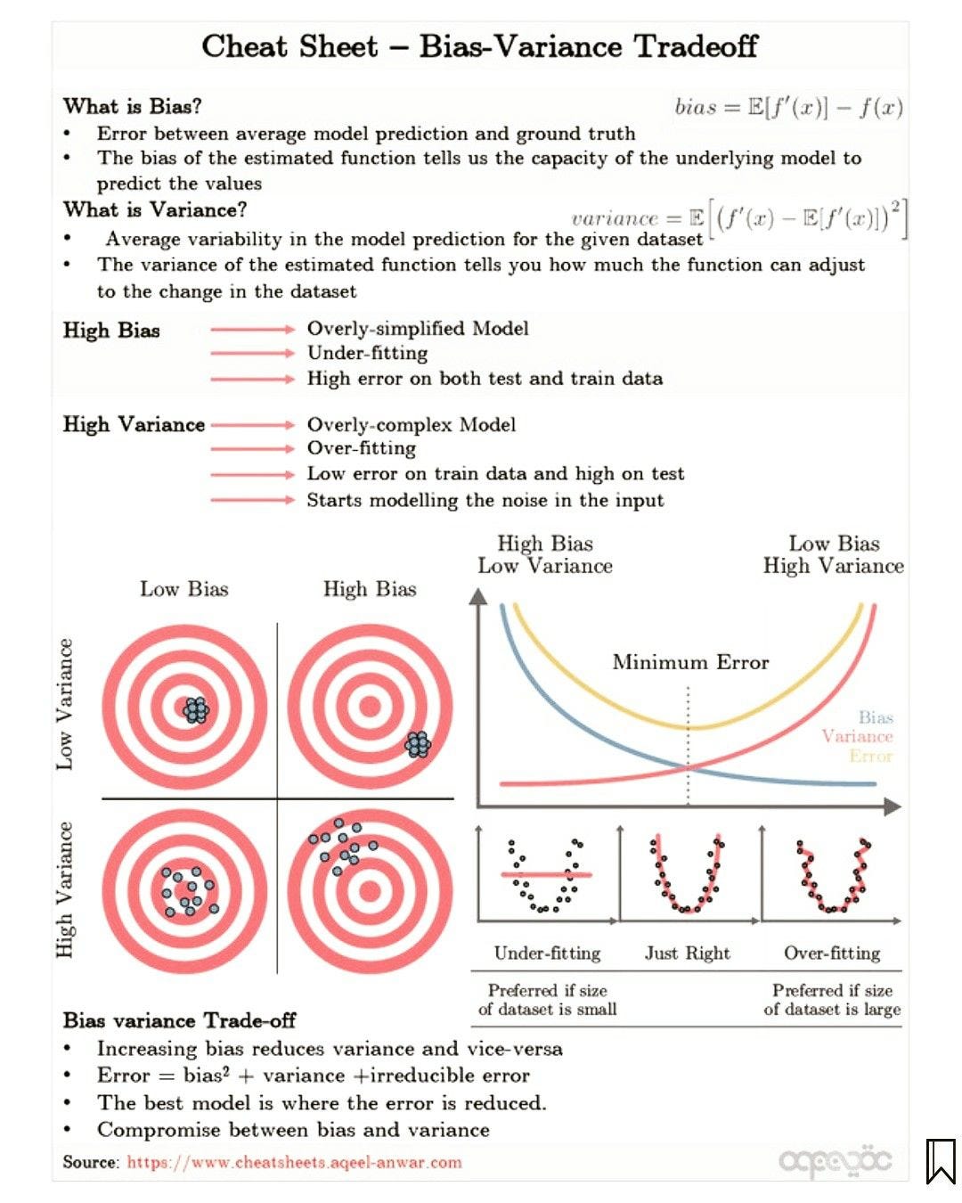
As you can see, the ideal scenario is low bias and low variance. The challenge in machine learning is that these two sources of error are often in opposition: decreasing one tends to increase the other.

Visualizing Underfitting and Overfitting

Let's explore this idea with a simple regression problem. Imagine trying to fit a model to a set of data points that have a non-linear relationship.

As you saw in the reading:

• A simple model (like a straight line) is too rigid. It has a high training error and a high test error. This is underfitting (high bias).
• A complex model (one that wiggles to hit every training point) has zero training error but a very high test error. It has memorized the noise in the training data and fails to generalize. This is overfitting (high variance).

The goal is to find a model complexity that is "just right"—one that captures the true underlying pattern without being swayed by the noise.

The Formal Decomposition of Error

Your desire to understand the "truthfulness" of these concepts requires us to move from intuition to a more rigorous, mathematical footing. We can formally decompose the expected squared error of a model at a single test point $x$.

Let's assume our true data-generating process is $y=f(x)+ϵ$, where $ϵ$ is random noise with a mean of zero and variance ${\sigma }^2$. Our goal is to learn a hypothesis $\hat{f}$ that approximates $f$. Since our learned model $\hat{f}$ depends on the specific training data $\mathcal{D}$ we receive, it is itself a random variable.

The expected prediction error at a point $x$, taken over all possible training sets $\mathcal{D}$ and the random noise $ϵ$ in the new data point, can be broken down as follows:

Let's break this down:

1. Bias²: The squared difference between the average prediction of our model (averaged over all possible training sets) and the true function value. This captures the systematic error of our modeling approach.
2. Variance: The expected squared difference between any single model's prediction and the average model prediction. This captures the instability of our model due to the specific training set.
3. Irreducible Error (${\sigma }^2$): The variance of the noise term $ϵ$. This error is inherent to the data itself and cannot be reduced by any model, no matter how good. This is the Bayes risk we discussed in the previous lesson.

The derivation of this decomposition is a classic result in statistical learning theory. The following video by Sebastian Raschka provides a clear, step-by-step walkthrough of the proof, which relies on a clever algebraic manipulation.

For an alternative presentation of the same derivation, you can also consult these notes from MIT.

The Tradeoff vs. Model Complexity

Now we can see precisely why this is a "tradeoff." As we increase the complexity of our model family $\mathcal{F}$ (e.g., using higher-degree polynomials, or deeper decision trees):

• Bias tends to decrease: A more flexible model is better able to approximate the true function $f(x)$.
• Variance tends to increase: A more flexible model is more likely to fit the noise in any particular training set, making it less stable across different datasets.

This relationship gives rise to the characteristic U-shaped curve for total test error when plotted against model complexity.

The Stanford Online video featuring Trevor Hastie provides an excellent series of examples illustrating this phenomenon.

Implications for Model Selection

The bias-variance tradeoff is not just a theoretical curiosity; it is the central challenge in model selection. While we can't directly calculate the true bias and variance (as they depend on the unknown function $f$ and the distribution $P$), the framework guides our strategy.

We control the tradeoff by tuning hyperparameters that govern model complexity.

• For K-Nearest Neighbors, the hyperparameter is K. A small K leads to a high-variance, low-bias model. A large K leads to a low-variance, high-bias model.
• For Decision Trees, complexity is controlled by hyperparameters like max_depth. A deep tree is high-variance, while a shallow tree is high-bias.

Ensemble methods are also designed around this tradeoff:

• Bagging (like in Random Forests) primarily aims to reduce the variance of high-variance models (like deep decision trees) by averaging their predictions.
• Boosting (like in Gradient Boosting Machines) primarily aims to reduce the bias by sequentially training simple models (like shallow trees) to correct the errors of their predecessors.

Let's return to the MLU-Explain article to see two concrete examples of controlling the tradeoff through hyperparameters.

Finally, the Python example in Sebastian Raschka's video (LINK) demonstrates how bagging can empirically reduce the variance of a decision tree regressor, a practical application of these theoretical ideas. You don't need to study the code in detail now, but it's valuable to see the outcome. He shows that a single decision tree has high variance, and a Bagging Regressor (an ensemble of trees) has a significantly lower variance, leading to better overall performance.

Conclusion

In this lesson, we have dissected model error into its core components, providing a rigorous foundation for understanding model performance.

Key Takeaways:

• Decomposition: The expected squared error of a model can be decomposed into three terms: $\text{Error}={\text{Bias}}^2+\text{Variance}+\text{Irreducible Error}$.
• Bias represents systematic error or how far the average model is from the truth. High bias causes underfitting.
• Variance represents model instability or its sensitivity to the specific training data. High variance causes overfitting.
• The Tradeoff: There is a fundamental tradeoff between bias and variance. Increasing model complexity typically decreases bias but increases variance.
• Model Selection: The goal of model selection is to find a level of complexity (often controlled by hyperparameters) that strikes an optimal balance between bias and variance, minimizing the total error on unseen data.

We now have a formal language to describe underfitting and overfitting. But how do we detect which problem our model is suffering from in a real-world scenario? In our next lesson, we will introduce learning curves, a practical diagnostic tool that allows us to visualize a model's training and validation performance to diagnose bias and variance issues.