In our last lesson, we built a foundational toolkit for evaluating classification models using the confusion matrix to derive metrics like precision and recall. We saw that these metrics often exist in a trade-off, and their values depend entirely on the specific classification threshold we choose. This raises a crucial question: how can we evaluate a model's performance independent of any single threshold?
This lesson will introduce a powerful technique to answer that question. Our goal is to plot a Receiver Operating Characteristic (ROC) curve and interpret the Area Under the Curve (AUC). You will learn how the ROC curve provides a complete picture of the trade-off between a model's benefits and costs across all possible thresholds. For you, aiming to master these concepts for teaching, understanding the deep probabilistic meaning of AUC will be a key focus.
From One Threshold to All of Them
Most classifiers, like logistic regression, don't just output a class label (e.g., "spam" or "not spam"). They output a probability of belonging to the positive class. We then use a threshold (often 0.5 by default) to make the final classification. As we saw with the precision-recall trade-off, this choice of threshold is significant.
Depending on the application, we might want to change this threshold.
- For a cancer screening test, we might lower the threshold to catch as many true cases as possible (maximizing recall), even if it means more false alarms (more false positives).
- For an email spam filter, we might raise the threshold to be very sure something is spam before moving it, minimizing the risk of losing an important email (maximizing precision).
This begs the question: how do we pick the best threshold? And more fundamentally, how can we assess a model's overall quality without committing to a single one? Trying to compare models by looking at dozens of confusion matrices for different thresholds would be incredibly inefficient. The StatQuest video below brilliantly illustrates this exact problem.
ROC and AUC, Clearly Explained!
This video from StatQuest with Josh Starmer masterfully sets the stage by showing how different thresholds lead to different confusion matrices and outcomes.
First, watch the review of how a threshold is used to create a confusion matrix from 02:01 to 04:43. Then, pay close attention to the segment from 04:43 to 06:54, which demonstrates the effect of changing this threshold and the challenge it creates for evaluation.
The Anatomy of an ROC Curve
The ROC curve offers an elegant solution by plotting the model's performance at all possible thresholds. It visualizes the trade-off between the "benefit" of finding true positives and the "cost" of flagging false positives.
The curve is plotted on a 2D graph with two key rates on its axes:
-
True Positive Rate (TPR) on the Y-axis: This is another name for Recall or Sensitivity, which you'll remember from our previous lesson. It answers: What proportion of the actual positives were correctly identified?
-
False Positive Rate (FPR) on the X-axis: This is a new metric for us. It answers: What proportion of the actual negatives were incorrectly identified as positive?
A perfect classifier would have a TPR of 1 (it finds all positives) and an FPR of 0 (it makes no false alarms). This corresponds to the top-left corner of the ROC space, (0, 1). A classifier that guesses randomly would, on average, have its TPR equal to its FPR. This is represented by the diagonal line from (0, 0) to (1, 1).
Let's ground these definitions in a formal source.
ROC Curves and AUC: The Ultimate Guide | Built In
This article from Built In provides clear definitions for the ROC curve and its axes, TPR and FPR, using a helpful analogy.
Please read the sections What Is ROC Curve? and True Positive Rate and False Positive Rate. The justice system analogy is a good way to frame the TPR vs. FPR trade-off.
Plotting the Curve: A Step-by-Step Visualization
So, how do we get from a set of predictions to this curve? The process involves calculating the (FPR, TPR) pair for every possible threshold and plotting these points. Imagine sorting all your data points by their predicted probability, from highest to lowest. You start with a threshold so high that you classify everything as negative (TPR=0, FPR=0). Then, you gradually lower the threshold, one data point at a time. Each time the threshold crosses the probability of a true positive, the TPR increases (the curve goes up). Each time it crosses the probability of a false positive, the FPR increases (the curve goes right).
The StatQuest video provides an exceptional step-by-step walkthrough of this exact process.
ROC and AUC, Clearly Explained!
This segment builds the ROC curve from scratch, one point at a time, making the construction process crystal clear.
Watch the video from 07:03 to 13:04. It will first formally define the axes and then meticulously plot the curve by varying the threshold and calculating the TPR and FPR at each step.
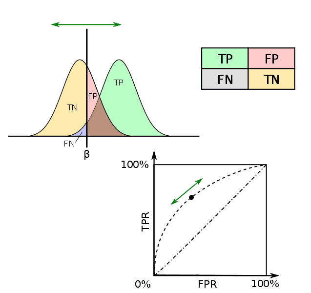
The image below beautifully synthesizes all these concepts. It shows the probability distributions for the negative (yellow) and positive (green) classes. The vertical line β is the decision threshold. By sliding this threshold, you change the areas corresponding to TP, FP, TN, and FN, which in turn traces out the ROC curve shown in the bottom panel.
Area Under the Curve (AUC): A Single Score for Performance
While the ROC curve provides a rich visualization, we often want a single number to summarize a model's performance and compare it to others. This is the purpose of the Area Under the Curve (AUC).
As the name suggests, AUC is simply the area under the ROC curve.
- An AUC of 1.0 represents a perfect classifier.
- An AUC of 0.5 represents a classifier with no discriminative ability, equivalent to random guessing (this is the area under the diagonal line).
- A good classifier will have an AUC between 0.5 and 1.0.
The Data School channel provides a great visual intuition for how the shape of the curve relates to the AUC score.
ROC Curves and Area Under the Curve (AUC) Explained
This video visually connects the separability of the classes to the shape of the ROC curve and the resulting AUC value.
Please watch the segment from 07:56 to 09:45. It clearly shows how a better classifier has a curve that "hugs" the top-left corner, resulting in a higher AUC.
The Deeper Meaning of AUC
AUC has a particularly elegant and important probabilistic interpretation that makes it a very popular metric. This is especially relevant given your goal to deeply understand these concepts.
The AUC is equal to the probability that the classifier will rank a randomly chosen positive instance higher than a randomly chosen negative instance.
This interpretation reveals why AUC is so powerful. It measures the model's ability to rank positive examples above negative ones, which is at the heart of what a good classifier should do. This property makes AUC independent of the chosen threshold and also insensitive to class imbalance, a major advantage over accuracy.
The Built In article we referenced earlier formally states this property.
ROC Curves and AUC: The Ultimate Guide | Built In
This section explains the properties of AUC, including its probabilistic interpretation and its invariance to threshold and scale.
Read the section What Is AUC?. Focus on the definition and the probabilistic meaning.
To truly solidify why this geometric area corresponds to this ranking probability, we can walk through an intuitive visual proof. Mochen's Blog provides an excellent step-by-step example. The core idea is that as you build the ROC curve on a grid, the area under the curve is the sum of rectangles formed each time you correctly classify a positive instance. The area of each rectangle represents the number of negative instances that this positive instance was correctly ranked above.
An Intuitive Explanation of ROC and AUC – Mochen's Blog
This article walks through a small example to build the ROC curve and then uses a clever visualization on a grid to "prove" the probabilistic meaning of AUC without formal math.
First, read through the setup in the section A Concrete Example. Then, follow the step-by-step construction of the curve in the section titled The ROC Curve. This reinforces the mechanical process of plotting. Finally, and most importantly, carefully read the section The AUC Measure. This provides the visual proof connecting the geometric area to the ranking probability.
Conclusion
In this lesson, we moved beyond single-threshold metrics to evaluate classification models holistically. By understanding and plotting the ROC curve, you can now visualize a model's performance across the entire spectrum of decision thresholds.
Key Takeaways:
- ROC curves plot the True Positive Rate (TPR) against the False Positive Rate (FPR) for all possible classification thresholds.
- A good model's ROC curve pushes towards the top-left corner, maximizing TPR while minimizing FPR. The diagonal line represents a random classifier.
- AUC (Area Under the Curve) quantifies this performance into a single number from 0.5 (random) to 1.0 (perfect).
- Crucially, AUC represents the probability that the model will rank a randomly chosen positive example higher than a randomly chosen negative one, making it a robust, threshold-independent metric.
With this, we have a comprehensive set of tools for evaluating supervised learning models. In our next lesson, we will shift gears to discuss k-fold cross-validation, a robust statistical method for using these evaluation metrics to estimate how well a model will generalize to new, unseen data.