Tree Traversal and Properties

1. Maximum Depth of a Binary Tree

The "maximum depth" (or height) of a binary tree is the length of the longest path from the root node down to the farthest leaf node. For this problem, we'll follow the common convention of counting the number of nodes on that path.

The Recursive DFS Approach

The most intuitive way to solve this is recursively. Think about it: the maximum depth of a tree is simply 1 (for the root itself) plus the maximum depth of its largest subtree (either left or right).

This gives us a very simple recursive relation:
maxDepth(node) = 1 + max(maxDepth(node.left), maxDepth(node.right))

The base case is a null node, which has a depth of 0.

This recursive breakdown is a fundamental pattern in tree algorithms. The following video provides a clear explanation and implementation of this approach, along with two iterative alternatives.

This image provides a great visualization of how the depth is calculated and passed up the call stack from the leaves to the root.

Alternative: The Iterative BFS Approach

Another intuitive way to find the maximum depth is to think of it as finding the total number of levels in the tree. Breadth-First Search (BFS) is perfect for this, as it explores the tree level by level. We can perform a standard level-order traversal and simply count how many levels we process.

While the recursive DFS is often the most concise code, the iterative BFS approach is also highly effective and avoids recursion depth limits, making it a robust solution. The video also covers an iterative DFS approach, which is good for completeness but less common in interviews for this specific problem.

2. Diameter of a Binary Tree

This is a slightly trickier, but extremely common, follow-up problem. The diameter of a binary tree is the length of the longest path between any two nodes. A critical point is that this path may or may not pass through the root. The length is measured by the number of edges.

The key insight is that for any given node, the longest path that passes through it is the sum of the maximum depth of its left subtree and the maximum depth of its right subtree. The tree's overall diameter is the maximum of these path lengths calculated for every node.

A naive O(N²) approach would be to iterate through every node, and for each one, calculate the depths of its left and right subtrees. We can do much better.

The Efficient O(N) Approach

The optimal solution involves a single post-order DFS traversal. We can write a helper function that does two things simultaneously:

1. Returns the maximum depth of the subtree rooted at the current node.
2. Updates a global or non-local variable to track the maximum diameter found so far. The diameter at the current node is left_depth + right_depth.

This "return one thing, update another" pattern is incredibly powerful.

Now, let's see this in action. The following video implements this exact logic.

Common Pitfall: A frequent mistake is confusing node count with edge count. For this problem, the diameter is the number of edges. If your depth/height function returns the number of nodes, the diameter through a node would be left_depth + right_depth. If your depth/height function returns the number of edges (i.e., height), the diameter is left_height + right_height. The NeetCode video is slightly different, using 2 + left + right because his height function for a null tree returns -1, which is a common trick to make the math work out. The core idea is the same: sum the path lengths down the left and right.

3. Balanced Binary Tree

A binary tree is height-balanced if, for every node in the tree, the absolute difference between the height of its left and right subtrees is no more than 1.

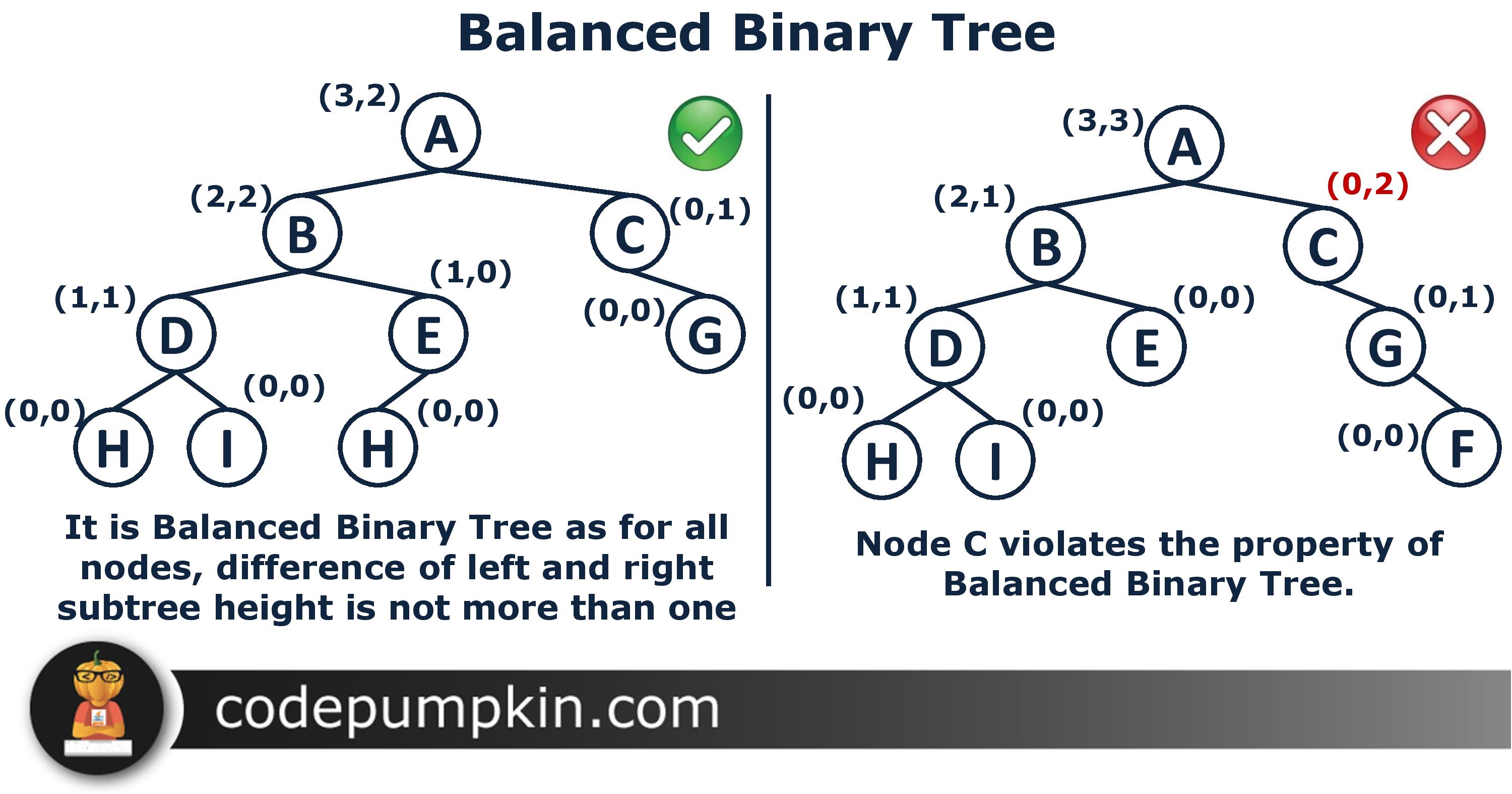
Just like with the diameter problem, we can devise an efficient O(N) solution using a single post-order traversal that avoids redundant height calculations.

The O(N) "Sentinel Value" Approach

The strategy is to create a DFS helper function that checks for balance as it calculates height.

• If a subtree is balanced, the function returns its height (a non-negative integer).
• If a subtree is unbalanced, the function immediately returns a special "sentinel" value, like -1, to signal this.

When a recursive call receives a -1 from one of its children, it knows the tree is unbalanced and can immediately stop and propagate the -1 up the call stack, enabling an early exit.

The core logic within the recursive helper function looks like this in Python:

def check_height(node):
    if not node:
        return 0  # Height of an empty tree

    # Recursively check left and right subtrees
    left_height = check_height(node.left)
    if left_height == -1:
        return -1  # Left subtree is unbalanced

    right_height = check_height(node.right)
    if right_height == -1:
        return -1  # Right subtree is unbalanced

    # Check the current node's balance
    if abs(left_height - right_height) > 1:
        return -1  # This node is unbalanced

    # If all is well, return the height of this subtree
    return 1 + max(left_height, right_height)

      A
     / \
    B   C
   / \ / \
  D  E F  G

Conclusion

Great job! You've just tackled three fundamental binary tree problems that are cornerstones of technical interviews. The real takeaway isn't just the solution to these three problems, but the underlying pattern.

Key Takeaways:

• Post-order Traversal is Powerful: Many tree property problems can be solved by computing information from child nodes first and then making a decision at the parent node.
• Dual-Purpose DFS: An efficient pattern is to use a single recursive DFS function that both returns a primary value (like height) and updates a secondary value (like diameter or a boolean flag) via a non-local/global variable or a sentinel return value.
• Complexity: All three problems can be solved optimally with O(N) time complexity, as we visit each node once, and O(H) space complexity for the recursion stack (where H is the tree's height).

In our next lesson, we'll continue using DFS to tackle another common category of tree problems: path-finding, such as finding a root-to-leaf path that sums to a specific value.