Analyzing Divide-and-Conquer Time Complexity

1. From Recursive Code to Recurrence Relations

Unlike iterative code where we can count loop runs, the complexity of a recursive function is defined in terms of itself. To analyze it, we first need to express its runtime as a recurrence relation.

A divide-and-conquer algorithm systematically breaks a problem into smaller subproblems, solves them recursively, and then combines their solutions. This process gives us a standard structure for our recurrence relation.

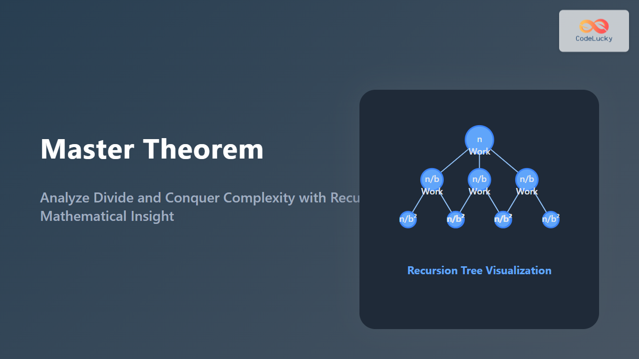
Let's use Merge Sort as our primary example. Its strategy is:

1. Divide: Split the array of size n into two halves. This takes constant time, O(1).
2. Conquer: Recursively call Merge Sort on each half. If the time to sort n elements is T(n), this step takes 2 * T(n/2).
3. Combine: Merge the two sorted halves back into a single sorted array. This requires looking at every element, so it takes linear time, O(n).

Combining these steps gives us the recurrence relation for Merge Sort:
$T(n)=2T(n/2)+O(n)$
This formula reads: "The time to sort n elements is equal to twice the time to sort n/2 elements, plus the O(n) time it takes to merge them."

Many common algorithms can be described this way. For example, Binary Search has the recurrence T(n) = T(n/2) + O(1) because it makes one recursive call on a problem half the size and does constant O(1) work for the comparison.

2. Building Intuition: The Recurrence Tree Method

Before we get to a formulaic solution, it's crucial to understand why these recurrences resolve to certain complexities. The recurrence tree method is a visual way to sum up all the work done by a recursive algorithm.

We'll visualize the recurrence T(n) = 2T(n/2) + cn (where cn is the work from O(n)).

1. Root Level: At the top, we have one problem of size n. The non-recursive work done at this level is cn.
2. Next Level: The root branches into two subproblems, each of size n/2. The work for each is c(n/2). The total work at this level is 2 * c(n/2) = cn.
3. And so on...: This continues until the problem size becomes 1 (the base case). At each level, the total work remains cn.

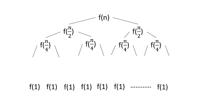
To get the total time, we need to answer two questions:

1. How much work is done at each level? (In this case, cn)
2. How many levels are there? (The tree's height)

Since we are repeatedly dividing n by 2 until we reach 1, the height of the tree is log₂(n).

So, the total work is (work per level) * (number of levels) = cn * log₂(n). In Big O notation, this is O(n log n).

To see this method applied to a concrete example, watch the following video. It provides a clear, step-by-step construction of a recurrence tree.

3. The Interview Shortcut: The Master Theorem

While the tree method provides great intuition, it can be slow in an interview. The Master Theorem is a powerful shortcut for solving recurrence relations that fit the common divide-and-conquer form:

$T(n)=aT(n/b)+f(n)$

Where:

• a ≥ 1 is the number of subproblems.
• b > 1 is the factor by which the input size is reduced (e.g., for n/2, b=2).
• f(n) is the cost of the work done outside the recursive calls (the "divide" and "combine" steps).

The theorem compares the work done in the recursive calls (represented by n^(log_b a)) with the work done at each level (f(n)). This tells us whether the complexity is dominated by the leaves of the recursion tree, the root, or is evenly distributed.

This leads to three cases:

1. Case 1: f(n) is "smaller" than n^(log_b a)
   If f(n) = O(n^(log_b a - ε)) for some constant ε > 0, then T(n) = Θ(n^(log_b a)).
   (Intuition: Most of the work happens in the vast number of subproblems at the leaves of the tree.)

2. Case 2: f(n) is "equal to" n^(log_b a)
   If f(n) = Θ(n^(log_b a) * log^k n) for some constant k ≥ 0, then T(n) = Θ(n^(log_b a) * log^(k+1) n).
   (Intuition: The work is spread evenly across all levels of the tree. The simplest sub-case, and most common in interviews, is when k=0, which gives T(n) = Θ(n^(log_b a) * log n).)

3. Case 3: f(n) is "larger" than n^(log_b a)
   If f(n) = Ω(n^(log_b a + ε)) for some constant ε > 0, and an additional "regularity condition" holds (a * f(n/b) ≤ c * f(n) for some constant c < 1), then T(n) = Θ(f(n)).
   (Intuition: Most of the work happens in the initial "combine" step at the root.)

The following video provides a very direct, example-driven explanation of these cases, which is perfect for memorizing the pattern for an interview.

Applying the Master Theorem: Examples

Let's apply this to the algorithms we've seen.

• Merge Sort: T(n) = 2T(n/2) + O(n)

  • a = 2, b = 2, f(n) = O(n).
  • Calculate log_b a = log₂2 = 1.
  • Compare f(n) with n^(log_b a) = n¹. They are asymptotically the same.
  • This is Case 2 (with k=0 since there is no log term in f(n)).
  • Result: T(n) = Θ(n¹ * log¹ n) = Θ(n log n).

• Binary Search: T(n) = T(n/2) + O(1)

  • a = 1, b = 2, f(n) = O(1).
  • Calculate log_b a = log₂1 = 0.
  • Compare f(n) with n^(log_b a) = n⁰ = 1. They are the same.
  • This is Case 2 (with k=0).
  • Result: T(n) = Θ(n⁰ * log¹ n) = Θ(log n).

• Strassen's Matrix Multiplication: T(n) = 7T(n/2) + O(n²)

  • a = 7, b = 2, f(n) = O(n²).
  • Calculate log_b a = log₂7 ≈ 2.81.
  • Compare f(n) = O(n²) with n^2.81. f(n) is polynomially smaller.
  • This is Case 1.
  • Result: T(n) = Θ(n^(log₂7)).

For a textual reference that lays out the Master Theorem and its limitations, you can review the following article.

Conclusion

Today we've added a crucial tool to your algorithm analysis toolkit. You've learned how to analyze recursive, divide-and-conquer algorithms, which are central to solving many interview problems efficiently.

Key Takeaways:

• Divide-and-conquer algorithms are modeled by recurrence relations of the form T(n) = aT(n/b) + f(n).
• The Recurrence Tree Method provides a visual intuition for how work is distributed in a recursive algorithm.
• The Master Theorem is a powerful shortcut for solving these recurrences by comparing f(n) to n^(log_b a), which tells you if the complexity is dominated by the root work, leaf work, or is balanced across the tree.
• You can now confidently analyze the runtime of key algorithms like Merge Sort (O(n log n)) and Binary Search (O(log n)).

In the next lesson, we will round out our foundational analysis skills by looking at space complexity. We'll explore how to account for memory usage, paying special attention to the difference between auxiliary space and the space consumed by the call stack in recursive algorithms—a direct and important follow-up to today's topic.