Shortest Path with BFS

1. The Core Idea of BFS: Exploring Level by Level

At its heart, Breadth-First Search is a systematic way to explore a graph. Imagine dropping a pebble into a pond; the ripples expand outwards one circle at a time. BFS does the same, starting from a source node and visiting all its immediate neighbors first (level 1), then all of their unvisited neighbors (level 2), and so on.

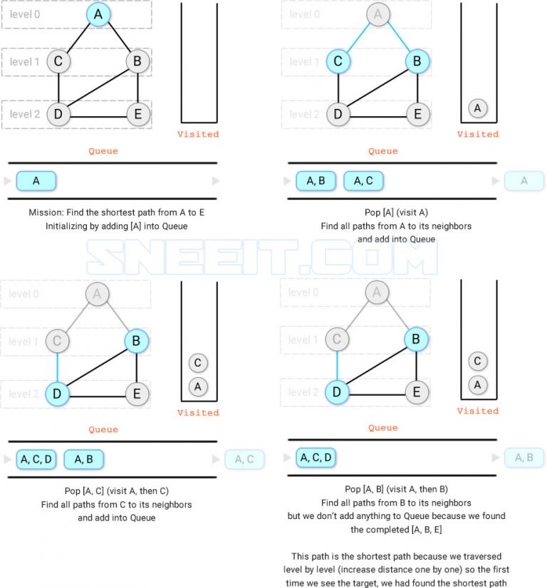
This level-by-level exploration is the key to why BFS is perfect for finding the shortest path in an unweighted graph. In an unweighted graph, the shortest path is simply the path with the fewest edges. Because BFS explores layer by layer, the very first time it reaches a destination node, it is guaranteed to have done so via a path with the minimum number of edges.

To build a strong intuition for this, watch the first part of the following video. It uses a great "balls with strings" analogy to visualize this level-by-level traversal.

2. The BFS Algorithm: Data Structures and Steps

To implement this level-by-level strategy, BFS relies on a few key data structures. Since you have a solid background in DSA, these should be familiar, but their roles in BFS are specific and important.

Let's summarize the roles of these components:

• Queue: This is the engine of BFS. It operates in a First-In, First-Out (FIFO) manner. We add a node's neighbors to the back of the queue and process nodes from the front. This ensures we finish exploring one "level" before starting the next.
• Visited Set: This is essential for efficiency and correctness. By tracking the nodes we've already visited (or added to the queue), we avoid redundant processing and prevent getting stuck in infinite loops in graphs with cycles.
• Predecessor (or Parent) Map: This is the key to our learning outcome. Simply traversing the graph isn't enough; we need to find the path. This map stores the "parent" of each node in the path (i.e., predecessor[neighbor] = current_node). Once we find our destination, we can backtrack through this map to reconstruct the shortest path.

With these data structures, the algorithm proceeds as follows. The video below provides a clear, animated walkthrough of these steps.

3. Implementing BFS for Shortest Path in Python

Now, let's translate this into Python code. Here is a function that finds the shortest path in an unweighted graph represented by an adjacency list. It returns the path as a list of nodes, or None if no path exists.

Notice how the code directly maps to the concepts we've discussed: queue, visited, and predecessor_map.

from collections import deque

def bfs_shortest_path(graph, start_node, end_node):
    """
    Finds the shortest path between start_node and end_node in an unweighted graph using BFS.

    Args:
        graph (dict): The graph as an adjacency list.
        start_node: The starting node.
        end_node: The target node.

    Returns:
        list: A list of nodes representing the shortest path, or None if no path exists.
    """
    if start_node not in graph or end_node not in graph:
        return None # Or raise an error

    # A deque is a highly efficient queue in Python
    queue = deque([start_node]) 
    
    # Keep track of visited nodes to avoid cycles
    visited = {start_node}
    
    # The predecessor map is key for reconstructing the path
    # format: {node: predecessor_node}
    predecessor_map = {start_node: None}

    while queue:
        current_node = queue.popleft()

        if current_node == end_node:
            # We found the target! Now, reconstruct the path.
            path = []
            node = end_node
            while node is not None:
                path.append(node)
                node = predecessor_map[node]
            return path[::-1] # Reverse the path to get start -> end

        for neighbor in graph.get(current_node, []):
            if neighbor not in visited:
                visited.add(neighbor)
                predecessor_map[neighbor] = current_node
                queue.append(neighbor)

    # If the queue becomes empty and we haven't found the end_node
    return None # No path exists

# --- Example Usage ---
# Let's use the graph from the GeeksforGeeks article
# V=8, E=10, S=2, D=6
edges = [
    [0, 1], [1, 2], [0, 3], [3, 4],
    [4, 7], [3, 7], [6, 7], [4, 5],
    [4, 6], [5, 6]
]
num_nodes = 8
adj_list = {i: [] for i in range(num_nodes)}
for u, v in edges:
    adj_list[u].append(v)
    adj_list[v].append(u)

start = 2
end = 6
path = bfs_shortest_path(adj_list, start, end)

print(f"Graph: {adj_list}")
print(f"Shortest path from {start} to {end}: {path}") 
# Expected Output: [2, 1, 0, 3, 4, 6]

Let's visualize the process for a simpler path, say from A to E.

4. Complexity Analysis

In an interview, after implementing an algorithm, you will always be asked about its complexity.

• Time Complexity: $O(V+E)$

  • Each vertex ($V$) is added to the queue and processed exactly once.
  • Every edge ($E$) is examined exactly once (or twice in an undirected graph, which is still proportional to $E$).
  • Therefore, the total time is proportional to the number of vertices plus the number of edges.

• Space Complexity: $O(V)$

  • In the worst case (e.g., a star graph where the center node is the source), the queue can hold up to $V-1$ nodes.
  • The visited set and predecessor_map will also store up to $V$ entries.
  • Thus, the space required scales linearly with the number of vertices.

5. Application: BFS on a Grid

A very common interview pattern is to ask a problem that can be modeled as a graph traversal on a 2D grid (like a maze or a pixel matrix). In these problems:

• Each cell is a vertex.
• Adjacent cells (up, down, left, right) are its neighbors.
• Obstacles (like walls) define which edges don't exist.

Finding the "shortest path" in a maze is a classic BFS problem. The "Flood Fill" algorithm, used in applications like MS Paint's bucket tool, is another great example.

Conclusion

Great job! You've just mastered one of the most fundamental and useful algorithms for your technical interviews. BFS is your go-to tool whenever a problem asks for the shortest path in an unweighted graph or involves level-by-level exploration.

Key Takeaways:

• BFS explores a graph level by level using a FIFO queue.
• It is guaranteed to find the shortest path in terms of the number of edges (for unweighted graphs).
• The implementation requires three key data structures: a queue for managing nodes to visit, a visited set to avoid redundant work, and a predecessor map to reconstruct the path.
• The time complexity is $O(V+E)$ and space complexity is $O(V)$.
• BFS is frequently applied to grid-based problems by treating cells as nodes and adjacent cells as neighbors.

Preview of the Next Lesson:

Now that we've covered breadth, it's time to explore depth. In our next lesson, we will implement Depth-First Search (DFS). While BFS uses a queue to go wide, DFS uses a stack to go deep. We'll compare its implementation and complexity to BFS and discover the unique set of problems where DFS is the more powerful tool.