Hello! Welcome to your next lesson on advanced graph data structures.
In our last lesson, we explored topological sorting for Directed Acyclic Graphs, a crucial pattern for problems involving dependencies and scheduling. As we previewed, we're now shifting our focus from directed graphs to a powerful tool often used with undirected graphs and dynamic connectivity problems: the Union-Find data structure.
Today's goal is to implement the Union-Find data structure with its essential optimizations: path compression and union by rank/size. This structure, also known as Disjoint Set Union (DSU), is a high-ROI pattern for technical interviews. It's the key to efficiently solving problems related to network connectivity, cycle detection in undirected graphs, and grouping related items. By the end of this lesson, you will have a complete, interview-ready implementation template.
1. What is Union-Find?
Imagine you have a collection of items, and you want to group them into a number of disjoint (non-overlapping) sets. The Union-Find data structure is designed to do two things very quickly:
- Find: Determine which set a particular item belongs to.
- Union: Merge two sets into a single new set.
Its primary application is to solve dynamic connectivity problems. For example, given a set of nodes in a graph, can we efficiently answer queries like "Are node A and node B connected?" while edges are being added to the graph dynamically? A naive DFS/BFS would be too slow if you have many queries. Union-Find provides a near-constant time solution.
To build a strong mental model, let's start with a short video that offers a great analogy and a high-level visual introduction.
This video from 'Hello Byte' introduces the core concepts of Union-Find using a company hierarchy analogy. It will help you visualize the structure and its basic operations.
Watch the first 6 minutes and 35 seconds of the video (from 00:00 to 06:35). Focus on understanding the three main operations (make_set, find, union) and how an array can be used to represent the parent-child relationships in the underlying tree structure.
As the video explains, we can represent these sets as a forest of trees, where each tree corresponds to a set. The root of the tree acts as the representative (or identifier) for that set.
- The
find(x)operation involves traversing from nodexup to the root of its tree. - The
union(x, y)operation merges the sets containingxandyby making the root of one tree a child of the root of the other.
2. The Need for Optimizations
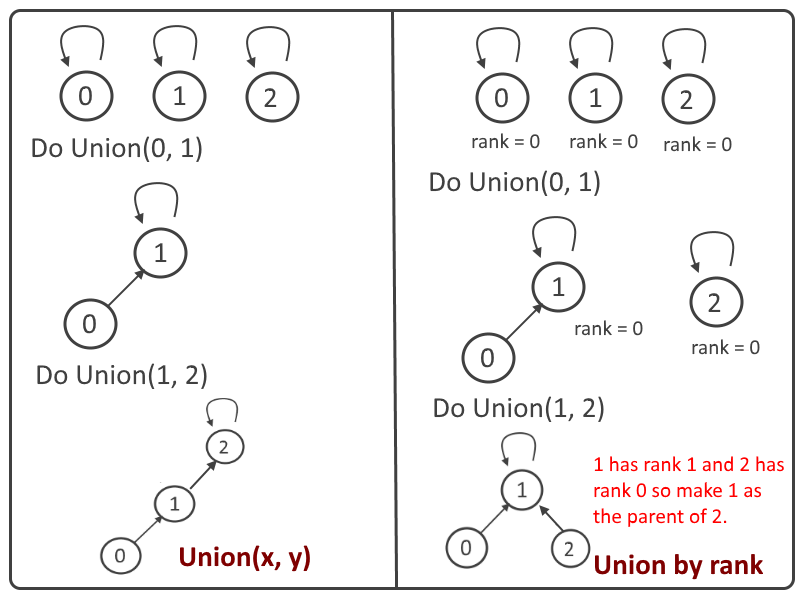
A simple implementation of this idea has a critical flaw. If we aren't careful about how we perform the union operation, we can end up creating very tall, skewed trees that resemble linked lists.
Consider uniting elements in a chain: union(0,1), then union(1,2), then union(2,3), and so on. The resulting tree would be a straight line. In this worst-case scenario, a find operation would have to traverse all the way up the chain, making its time complexity . For interview settings where performance is key, this is unacceptable.
To achieve the near-constant time complexity that makes Union-Find so powerful, we need two optimizations.
3. The Key Optimizations: Path Compression and Union by Rank/Size
These two techniques work together to keep the trees in our forest extremely flat, ensuring that the find operation remains fast.
Union by Rank / Union by Size
This optimization applies to the union operation. Instead of arbitrarily attaching one tree to another, we use a heuristic to decide which tree goes under which.
- Union by Rank: We keep track of the "rank" of each root, which is an upper bound on the height of its tree. When uniting two trees, we always attach the root of the shorter tree (lower rank) to the root of the taller tree (higher rank). This prevents the overall tree height from growing unnecessarily. If the ranks are equal, we can pick one, attach the other, and increment the rank of the new root.
- Union by Size: This is a similar, often more intuitive, alternative. We track the number of nodes (size) in the set represented by each root. When uniting, we attach the root of the smaller set to the root of the larger set.
Path Compression
This optimization applies to the find operation. When we call find(x), we traverse the path from x up to its root. Path compression does a simple, brilliant thing: after finding the root, it makes every node along that path a direct child of the root.

With these two optimizations combined, the amortized time complexity of both union and find operations becomes nearly constant, specifically , where is the Inverse Ackermann function. This function grows so slowly that for any practical input size N, it's less than 5.
Let's watch a detailed walkthrough of implementing these optimizations.
G-46. Disjoint Set | Union by Rank | Union by Size | Path Compression
This comprehensive video from 'take U forward' dives deep into the implementation details of both optimizations. It provides a step-by-step trace of how the data structure evolves.
Please watch two segments from this video: Union by Rank & Path Compression (05:13 - 22:07): This part explains the logic of Union by Rank and Path Compression in detail. Pay close attention to how the parent and rank arrays are updated. Union by Size (35:12 - 41:07): This segment introduces Union by Size as an alternative. Notice how it's conceptually similar to Union by Rank but uses a size array instead.
4. Implementation Template
Now, let's consolidate everything into a clean, reusable Python class. This template is what you should aim to reproduce in an interview. You will see it implements the logic discussed in the video.
We will have a class UnionFind that is initialized with the number of elements n. It will maintain a parent array and either a rank or size array.
__init__(self, n): Initializesparent[i] = ifor all elements, and sets their initialrankto 0 orsizeto 1.find(self, i): Finds the root ofiand performs path compression using recursion.union(self, i, j): Merges the sets containingiandjusing union by rank or union by size.
The following resource provides excellent, clean code for both variations.
Union By Rank and Path Compression in Union-Find ...
This GeeksForGeeks article provides complete, optimized implementations of Union-Find in multiple languages. We will focus on the Python code as it serves as a perfect template.
Study the Python code snippets for both 'Union by Rank' and 'Union by Size'. Take note of the recursive implementation of find() for path compression and the logic within the unionSets()/unionBySize() methods. You don't need to read the whole article, just focus on understanding these code blocks.
Here's a summary of the Union by Size implementation, which is a very common interview choice:
class UnionFind:
    def __init__(self, n):
        # Each node is its own parent initially
        self.parent = list(range(n))
        # Each component has a size of 1 initially
        self.size = [1] * n

    def find(self, i):
        # Base case: if i is its own parent, it's the root
        if self.parent[i] == i:
            return i

        # Recursive call to find the root, with path compression
        self.parent[i] = self.find(self.parent[i])
        return self.parent[i]

    def union(self, i, j):
        # Find the roots of the sets containing i and j
        root_i = self.find(i)
        root_j = self.find(j)

        # If they are already in the same set, do nothing
        if root_i != root_j:
            # Union by size: attach the smaller tree to the root of the larger tree
            if self.size[root_i] < self.size[root_j]:
                root_i, root_j = root_j, root_i # Ensure root_i is the larger set

            self.parent[root_j] = root_i
            self.size[root_i] += self.size[root_j]
            return True # Return True to indicate a successful merge

        return False # Return False if they were already connected
Test your understanding!
Imagine you have a UnionFind structure for 5 elements (0-4), implemented with Union by Rank and Path Compression. The parent array is [0, 1, 2, 3, 4] and the rank array is [0, 0, 0, 0, 0].
Trace the state of the parent and rank arrays after these operations:
union(0, 1)union(2, 3)union(0, 2)
What are the final parent and rank arrays?
Show answer
-
union(0, 1):find(0)-> 0.find(1)-> 1.- Ranks are equal (both 0). Attach 1 to 0.
parentbecomes[0, 0, 2, 3, 4].rankbecomes[1, 0, 0, 0, 0](rank of root 0 increases).
-
union(2, 3):find(2)-> 2.find(3)-> 3.- Ranks are equal (both 0). Attach 3 to 2.
parentbecomes[0, 0, 2, 2, 4].rankbecomes[1, 0, 1, 0, 0](rank of root 2 increases).
-
union(0, 2):find(0)-> 0.find(2)-> 2.rank[0]is 1,rank[2]is 1. Ranks are equal. Attach 2 to 0.parentbecomes[0, 0, 0, 2, 4].rankbecomes[2, 0, 1, 0, 0](rank of root 0 increases).
Final State:
parent:[0, 0, 0, 2, 4]rank:[2, 0, 1, 0, 0]
Conclusion
You have now built one of the most efficient data structures for handling dynamic connectivity. Its elegance and performance make it a favorite in competitive programming and a valuable tool for your interview arsenal.
Key Takeaways:
- Union-Find (DSU) is specialized for managing disjoint sets and answering connectivity queries.
- A naive implementation leads to performance, which is too slow.
- Union by Rank/Size keeps the underlying trees flat during
unionoperations. - Path Compression flattens the tree structure during
findoperations. - Together, these optimizations give Union-Find a nearly constant amortized time complexity ().
- The space complexity is to store the
parentandrank/sizearrays.
This table from the "Union-Find" chapter in shawonnotes is a great summary of when to use this data structure.
| Problem Type | Union-Find? | Why? |
|---|---|---|
| Connected Components | ✅ Yes | Efficient for merging nodes dynamically. |
| Cycle Detection (Undirected) | ✅ Yes | Detects cycles in O(1) amortized operations. |
| Cycle Detection (Directed) | ❌ No | Use DFS or Kahn’s Algorithm instead. |
| Kruskal’s Algorithm (MST) | ✅ Yes | Quickly processes edge unions. |
| Dynamic Path/Connectivity Queries | ✅ Yes | Answers connectivity in O(1) amortized time. |
Preview of the Next Lesson:
Now that you have mastered the implementation of the Union-Find data structure, our next lesson will focus on its practical application. We will apply Union-Find to efficiently solve common graph connectivity problems, such as counting the number of connected components in a graph and detecting redundant connections. You'll see just how powerful this tool is in action.