Finding the Lowest Common Ancestor in a BST

What is a Lowest Common Ancestor?

The Lowest Common Ancestor (LCA) between two nodes, p and q, in a tree is defined as the lowest (i.e., deepest) node that has both p and q as descendants. A node can be a descendant of itself.

Let's look at a visual example.

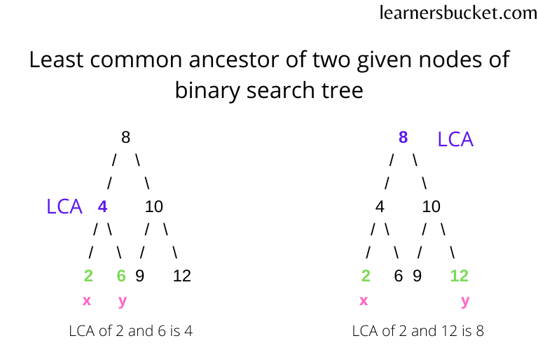
For a general binary tree, a common approach is to find the path from the root to p and the path from the root to q, and then find the last common node in both paths. This works, but it's inefficient, requiring $O(N)$ time and $O(N)$ space in the worst case. For a BST, we can do much better.

The Key Insight: Leveraging the BST Property

The defining property of a BST is that for any given node, all values in its left subtree are smaller, and all values in its right subtree are larger. We can use this to our advantage.

Imagine you are at the root of the tree, looking for the LCA of p and q. There are three possibilities:

1. Both p and q have values smaller than the current node's value. This means the LCA must be in the left subtree.
2. Both p and q have values larger than the current node's value. This means the LCA must be in the right subtree.
3. The values of p and q split at the current node: one is smaller (or equal) and one is larger (or equal). This means the current node is the "fork in the road." It's the first ancestor from the top that has p and q in different subtrees. Therefore, the current node is the LCA. This case also handles the situation where one of the target nodes is the ancestor of the other.

This logic allows us to discard half of the tree at each step, similar to binary search.

To see this logic in action, let's watch a short video that explains it visually.

The Algorithm: Iterative Approach

As the video demonstrates, this logic translates into a highly efficient iterative algorithm. This approach is generally preferred in interviews because it uses constant extra space.

Here is the algorithm:

1. Start with a pointer, current, at the root of the tree.
2. Loop as long as current is not null.
3. If both p.val and q.val are greater than current.val, move to the right child: current = current.right.
4. If both p.val and q.val are less than current.val, move to the left child: current = current.left.
5. If neither of the above is true, it means we've found the split point (or one of the nodes is the LCA). The current node is the LCA, so we return it.

Let's see the code implementation of this.

Here is the Python code for your reference. It's a pattern worth committing to memory.

# Definition for a binary tree node.
# class TreeNode:
#     def __init__(self, x):
#         self.val = x
#         self.left = None
#         self.right = None

class Solution:
    def lowestCommonAncestor(self, root: 'TreeNode', p: 'TreeNode', q: 'TreeNode') -> 'TreeNode':
        current = root
        
        while current:
            # If both p and q are greater than parent
            if p.val > current.val and q.val > current.val:
                current = current.right
            # If both p and q are smaller than parent
            elif p.val < current.val and q.val < current.val:
                current = current.left
            # We have found the split point, i.e. the LCA
            else:
                return current

Alternative: Recursive Approach

The same logic can be implemented recursively. The code is often more concise, but it comes at the cost of using extra space on the call stack.

Here's the recursive Python code from the article:

def LCA(root, n1, n2):
    if root is None:
        return None

    # If both n1 and n2 are smaller than root, LCA lies in left
    if root.data > n1.data and root.data > n2.data:
        return LCA(root.left, n1, n2)

    # If both n1 and n2 are greater than root, LCA lies in right
    if root.data < n1.data and root.data < n2.data:
        return LCA(root.right, n1, n2)

    # If we reach here, then root is the LCA
    return root

Complexity Analysis

Let's quickly summarize the performance, which is the main reason this approach is so powerful.

• Time Complexity: $O(H)$, where $H$ is the height of the tree. At each level, we make one decision and eliminate the rest of the tree at that level. For a balanced BST, this becomes $O(\log N)$. In the worst case (a skewed tree), it's $O(N)$.
• Space Complexity:
  • Iterative: $O(1)$ — We only use a few pointers, regardless of the tree's size. This is optimal.
  • Recursive: $O(H)$ — Due to the recursion call stack. For a balanced BST, this is $O(\log N)$; for a skewed tree, $O(N)$.

This is a significant improvement over the $O(N)$ time and space complexity of the naive approach for a general binary tree.

Conclusion

In this lesson, we tackled another fundamental BST problem, perfect for technical interviews. You've learned how to exploit the BST ordering property to find the Lowest Common Ancestor efficiently.

Key Takeaways:

• The LCA in a BST is the "split point" node, where the paths to the two target nodes diverge.
• The search for the LCA can be done in $O(H)$ time by traversing from the root and deciding at each node whether to go left, go right, or stop.
• The iterative solution is generally preferred due to its optimal $O(1)$ space complexity.
• Be prepared to explain why this approach is superior to methods used for general binary trees.

In our next and final lesson on BSTs, we'll address another common problem: constructing a height-balanced BST from a sorted array. This will tie together concepts of tree balance and BST properties. See you then