Hash Tables: Fundamentals, Functions, and Collision Resolution

1. The Need for Speed: Beyond Arrays

Imagine you're building a system to manage user profiles. You want to retrieve a user's data using their unique username.

If you store the profiles in an array or list, finding a user by their username would require a linear search—iterating through the array one by one. This is an $O(n)$ operation, which becomes prohibitively slow as the number of users grows. We need a way to get directly to the data, much like using an index to access an element in an array in $O(1)$ time.

This is the problem hash tables were designed to solve. They provide a mechanism to map a key (like a username) to a value (the user profile) with an average time complexity of $O(1)$ for lookups, insertions, and deletions.

2. The Core Components: Hash Functions and Buckets

So, how does a hash table convert a key (like the string "johndoe") into an array index? This is done through a two-step process involving a hash function and the modulo operator.

The Hash Function

A hash function is a special algorithm that takes an input key and transforms it into an integer, known as a hash code.

A good hash function should have these properties:

• Deterministic: The same key must always produce the same hash code.
• Uniform Distribution: It should spread keys out as evenly as possible across the potential hash codes to avoid bunching them together.
• Fast: The computation itself should be very quick.

For example, a simple (though not very good) hash function for a string could be to sum the ASCII values of its characters.

From Hash Code to Array Index

The hash code produced can be a very large number. To map it to an index within our underlying array of a fixed size m, we use the modulo operator (%).

This calculation guarantees that the resulting index will be within the bounds of our array, from 0 to m-1. Each slot in this array is often called a bucket.

While the simple "remainder method" is easy to understand, more sophisticated hash functions exist, like the folding method (breaking the key into chunks and adding them) or the mid-square method (squaring the key and extracting the middle digits). You can explore these further in the "Hashing" article from Runestone Academy (resource ID LINK), under the section "Hash Functions."

3. The Inevitable Problem: Collisions

What happens if two different keys produce the same index? For example, using a table of size 11 and the remainder method, both keys 23 and 34 would map to index 1 (23 % 11 = 1 and 34 % 11 = 1). This is called a collision.

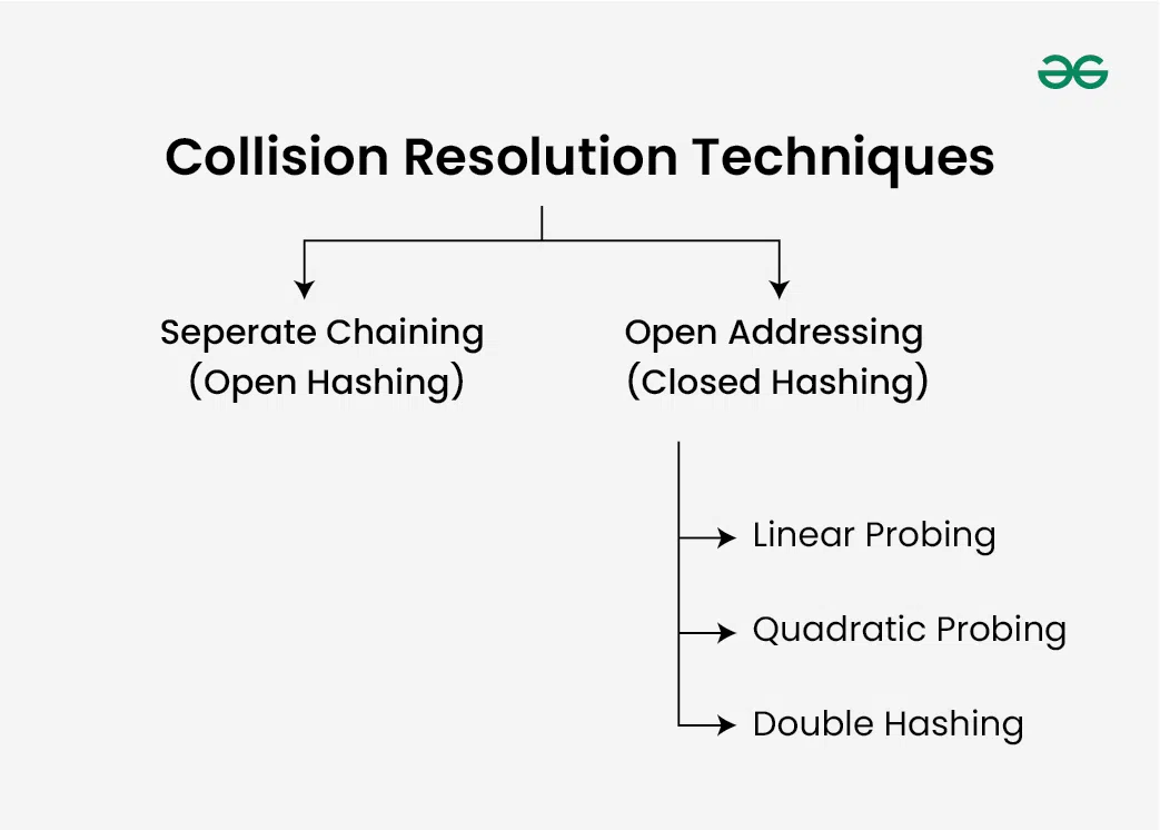
Since the number of possible keys is usually far greater than the number of available buckets, collisions are a fact of life. A robust hash table implementation must have a strategy to handle them. These strategies are broadly divided into two categories: Separate Chaining and Open Addressing.

4. Collision Resolution Strategy 1: Separate Chaining

This is the most common collision resolution strategy. The idea is simple: instead of each bucket holding just one value, it holds a pointer to another data structure—typically a linked list—that stores all the key-value pairs that hashed to that index.

• Insertion: When a collision occurs, you simply append the new key-value pair to the linked list at that bucket.
• Lookup: You hash the key to find the correct bucket, then perform a quick search through the small linked list to find the key you're looking for.

The Tradeoff: Chaining is simple to implement and handles a high density of elements gracefully. However, in the worst-case scenario where a poor hash function maps all keys to the same bucket, the hash table degrades into a single linked list, and all operations become $O(n)$.

5. Collision Resolution Strategy 2: Open Addressing

In open addressing, all key-value pairs are stored directly within the main array. When a collision occurs, the algorithm probes for the next available bucket according to a fixed sequence.

There are three common probing techniques:

1. Linear Probing: If a collision occurs at index, check index + 1, then index + 2, and so on, until an empty bucket is found.

   • Problem: This can lead to primary clustering, where long runs of occupied buckets form, degrading performance as insertions and lookups have to traverse these clusters.

2. Quadratic Probing: Instead of stepping linearly, you check index + 1^2, index + 2^2, index + 3^2, etc. This helps break up the large clusters formed by linear probing.

3. Double Hashing: A second hash function is used to determine the step size for probing. This is the most effective at avoiding clustering but is also the most complex to implement.

6. Managing Performance: Load Factor and Rehashing

The performance of a hash table is highly dependent on how full it is. We measure this with the load factor, $\lambda$.

As $\lambda$ increases, the probability of collisions rises, and performance suffers. To combat this, hash tables automatically resize themselves. When the load factor exceeds a certain threshold (typically around 0.7 for open addressing), a process called rehashing occurs:

1. A new, larger array is created (often double the size).
2. All existing key-value pairs are iterated over, and their hashes are re-calculated for the new array size.
3. Each element is inserted into its new position in the larger array.

Rehashing is an $O(n)$ operation, which can cause a temporary performance spike. However, since it happens infrequently, the cost is amortized over many insertions, and the average (amortized) time complexity for insertion remains $O(1)$.

To consolidate your understanding of these collision strategies, the following resource provides an excellent summary.

Conclusion

You've just completed a deep dive into the engine room of one of computing's most important data structures. While you'll rarely implement a hash table from scratch in an interview, knowing what's happening under the hood is non-negotiable for a strong candidate.

Key Takeaways:

• Purpose: Hash tables provide $O(1)$ average time for inserts, deletes, and lookups by mapping keys to array indices.
• Mechanism: A hash function computes a hash code from a key, and the modulo operator maps that code to a bucket in an array.
• Collisions: They are inevitable. The two main resolution strategies are Separate Chaining (linked lists in each bucket) and Open Addressing (probing for the next free bucket).
• Performance: The load factor measures how full the table is. Rehashing to a larger array is done to keep the load factor low and maintain $O(1)$ amortized performance. The worst-case performance for all operations is $O(n)$.

In our next lesson, we will move from theory to practice. You'll learn how to apply hash maps and hash sets to solve a very common category of interview problems: frequency counting.