Model Training and Comparison

In our last lesson, we constructed a complete preprocessing and feature engineering pipeline—an automated "factory" for preparing raw data. With this critical piece of infrastructure in place, we can now turn our attention from data preparation to model experimentation. This lesson addresses the heart of applied machine learning: training, evaluating, and systematically comparing multiple candidate models.

You've learned about a diverse set of algorithms, each with unique strengths and mathematical underpinnings. But how do you choose the best one for your specific problem? The answer is to test them empirically. We'll build a "test harness" to run a suite of models through the same evaluation process, ensuring a fair and rigorous comparison. This practice of systematic evaluation is fundamental to moving from academic knowledge to professional, results-driven data science.

Why Test Multiple Models?

Different algorithms create fundamentally different decision boundaries. A linear model like Logistic Regression will find a straight line, while a K-Nearest Neighbors or a tree-based model can capture complex, non-linear patterns. There's rarely a single "best" algorithm for all problems; the data's underlying structure dictates which model will perform best.

The image below vividly illustrates this. It shows how ten different classifiers approach the same three datasets. Notice how some models excel on one data structure but fail on another.

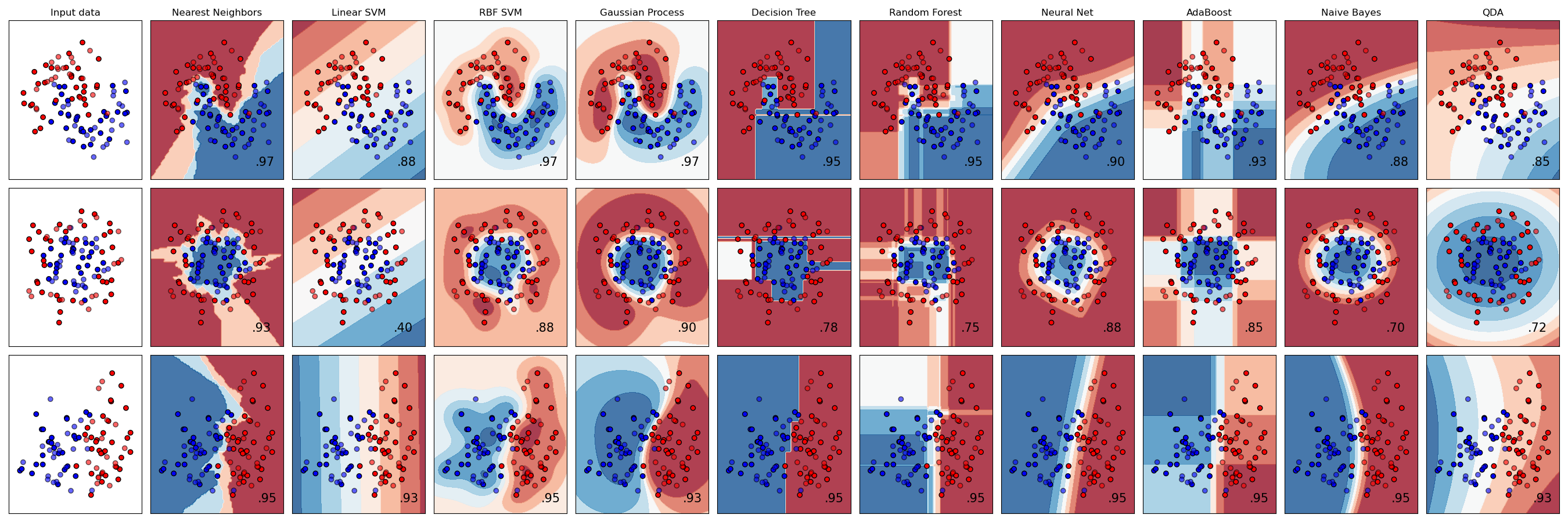
This grid shows the decision boundaries for ten different classifiers on three synthetic datasets. Notice how models like Linear SVM struggle with non-linear shapes, while RBF SVM, Random Forest, and Gaussian Process handle them with ease. This visualizes why testing multiple models is crucial.

This highlights the necessity of a "bake-off"—a competition to see which model, when applied to your data, yields the best results.

Creating a Consistent Test Harness

To compare models fairly, you must evaluate them under identical conditions. This means using:

The exact same dataset.
The exact same preprocessing steps (our pipeline from the last lesson!).
The exact same evaluation procedure.

A simple train-test split is often not robust enough for model comparison because the results can be sensitive to how the split was made. A much better approach, as you learned previously, is k-fold cross-validation. It provides a more stable estimate of a model's performance on unseen data by training and testing on multiple different splits of the data.

The following video from the codebasics channel offers an excellent refresher on this concept and demonstrates why a single split can be misleading. It also introduces the highly convenient cross_val_score function in scikit-learn, which is the workhorse of our test harness.

Machine Learning Tutorial Python 12 - K Fold Cross Validation

This video explains the motivation for k-fold cross-validation and demonstrates how to use the cross_val_score function to simplify model evaluation.

Watch the introduction to understand the pitfalls of using a single train-test split for evaluation. Then, skip ahead to the section on cross_val_score which shows how this single function can replace the entire manual loop of splitting data, training, and scoring.

The key takeaway is that cross_val_score automates the k-fold process, returning an array of scores (one for each fold), which we can then use to assess both the average performance and the consistency of each model.

A Practical Template for Model Comparison

Now, let's put these concepts into a practical script. We will create a test harness that:

Defines a list of candidate models.
Loops through each model.
Evaluates each model using 10-fold cross-validation with cross_val_score.
Collects the results.
Presents a comparison both numerically and visually.

The following article from Machine Learning Mastery provides a perfect, concise template for this entire process. While the example doesn't use a Pipeline object, you can imagine that the model variable in their code would be your full pipeline (e.g., Pipeline(steps=[('preprocessor', preprocessor), ('classifier', LogisticRegression())])).

How To Compare Machine Learning Algorithms in Python ...

This article presents a clear and effective template for creating a test harness to compare multiple machine learning algorithms.

First, read the brief section on consistent comparison to reinforce the core idea. Then, carefully study the complete Python script. This is your blueprint. Pay attention to how it: Loads the data (in your case, this would be your training data). Creates a list of (name, model) tuples to define the candidates. Loops through this list, calling model_selection.cross_val_score for each one. Appends the resulting array of scores from the folds into a results list. Prints the mean and standard deviation for each model. Uses matplotlib to create a box plot for visual comparison. Finally, review the results section, which shows the numerical output and the resulting box plot.

Interpreting the Results

The script from the article produces two crucial outputs for comparison:

Numerical Summary: A list showing the mean accuracy and standard deviation for each model across the cross-validation folds. The mean gives you the average performance, while the standard deviation tells you how consistent that performance is. A low standard deviation is desirable, as it suggests the model's performance doesn't vary wildly depending on the training data.
Box Plot Visualization: This is arguably the most important output. A box plot visualizes the distribution of the accuracy scores from each fold.

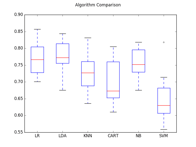
A box plot comparing the cross-validation accuracy scores for six different algorithms. The red line indicates the median accuracy, the box represents the interquartile range (IQR, the middle 50% of scores), and the whiskers show the full range of scores. This allows for a quick comparison of both central tendency (median) and variance (box/whisker size).

From this plot, you can see not only which algorithms have a higher median accuracy (LR, LDA) but also which ones are more stable (NB has a very tight distribution) and which are more variable (SVM has a wide range of outcomes). This rich visualization is far more informative than a single accuracy number.

The "Data Professor" YouTube channel provides another excellent, hands-on walkthrough of this entire process, culminating in a similar comparison using a pandas DataFrame and a seaborn bar plot. This is a great alternative way to organize and visualize your findings.

Compare Machine Learning Classifiers in Python

This video provides a complete walkthrough of comparing 14 different classifiers on a synthetic dataset.

You can skim through the video to see the workflow in action: He imports and initializes a long list of classifiers. He then iterates through the models, training and scoring each one on a single test set. (Note: using cross-validation as shown in the article is a more robust approach). Finally, he demonstrates a great way to organize and visualize the results using a pandas DataFrame and a seaborn bar plot, which provides a clean and readable comparison.

Beyond a Single Metric: A Holistic Comparison

While accuracy is a good starting point, a professional model evaluation considers multiple factors. As you know from our lesson on classification metrics, precision, recall, and F1-score often tell a more complete story, especially with imbalanced datasets.

Furthermore, model selection isn't just about predictive performance. You must also consider:

Training Time: How long does it take to train the model? This is critical for large datasets or applications requiring frequent retraining.
Prediction Latency: How fast can the trained model make predictions?
Interpretability: Can you explain why the model made a certain prediction?
Tuning Effort: How sensitive is the model to its hyperparameters? A model that works well out-of-the-box is often preferred over one that requires extensive tuning.

The following article from DataCamp provides an excellent real-world comparison between Random Forest and XGBoost, looking beyond simple accuracy.

Ensemble Learning in Python: A Hands-On Guide to ...

This section of the article compares Random Forest and XGBoost on the Dry Beans dataset, providing a fantastic example of a multi-faceted model comparison.

Please read the section Random Forest vs XGBoost. Pay close attention to the tables that compare the models on multiple metrics, including accuracy and macro F1-score. Also, note the qualitative comparison in the final table, which considers factors like tuning effort and dataset size.

This holistic approach is what separates good data scientists from great ones. The goal of the model comparison stage is not just to find the model with the highest accuracy, but to gather the evidence needed to select the model that best fits the overall project requirements.

Conclusion

In this lesson, you've learned how to bridge the gap between having a preprocessed dataset and selecting a promising model. By creating a standardized test harness, you can rigorously and fairly evaluate multiple algorithms.

Key Takeaways:

Use a Test Harness: A consistent framework for evaluation is essential for a fair comparison of machine learning models.
Leverage Cross-Validation: Use scikit-learn's cross_val_score to get a robust estimate of each model's performance and stability.
Visualize Your Results: Box plots are an excellent tool for comparing the distribution of cross-validation scores, revealing both median performance and variance.
Compare Holistically: Your final decision should not be based on a single metric. Consider a range of performance metrics, along with practical factors like training time, interpretability, and tuning complexity.

What's Next:

You now have a ranked list of candidate models and a wealth of data about their performance. In our next and final lesson of this project, you will synthesize all this information to select and justify the choice of a final model based on the performance metrics and the specific requirements of the problem. This is the last step before finalizing your modeling approach.