Naive Bayes: Gaussian, Multinomial, and Bernoulli

A Map of Naive Bayes Classifiers

The fundamental difference between the Naive Bayes variants lies in the assumption they make about the distribution of your features. The choice of classifier is therefore not arbitrary; it's a direct consequence of the data you are working with.

Let's start with a high-level overview.

As the diagram illustrates, the core decision boils down to the type of data in your feature columns:

• Are your features continuous (e.g., age, height, temperature)? You'll likely use Gaussian Naive Bayes.
• Are your features discrete counts (e.g., the number of times a word appears in an email)? This is the domain of Multinomial Naive Bayes.
• Are your features binary—simply indicating presence or absence (e.g., does a specific word appear in a document: yes/no)? This calls for Bernoulli Naive Bayes.

Let's now examine each of these in more detail.

Gaussian Naive Bayes: For Continuous Features

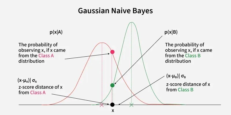
When your dataset contains continuous features like measurements, sensor data, or financial metrics, you can't calculate probabilities based on simple frequency counts. Instead, Gaussian Naive Bayes assumes that for any given class, the continuous features follow a Gaussian (or normal) distribution.

Given your background in probability and statistics, you'll recognize the normal distribution as the familiar "bell curve." To calculate the likelihood $P(x_i|y)$ for a feature $x_i$ and a class $y$, the algorithm first estimates the mean (${\mu }_y$) and variance (${\sigma }_y^2$) of that feature for all samples belonging to class $y$ in the training data.

Then, for a new data point, it uses the probability density function (PDF) of the Gaussian distribution to find the likelihood of that feature value occurring for that class:

You don't need to memorize this formula, but you should understand its role: it provides a "likelihood score" for a continuous value based on how close it is to the mean of that class. A value closer to the mean will have a higher likelihood.

Common Use Cases:

• Medical diagnosis based on continuous measurements (e.g., blood pressure, cholesterol levels).
• Classifying species in the Iris dataset based on petal and sepal length/width.
• Financial modeling where features might include stock prices or economic indicators.

Multinomial Naive Bayes: For Discrete Counts

This is the variant we implicitly discussed in the previous lesson with the spam filter example. Multinomial Naive Bayes is designed for features that represent discrete counts.

The classic use case is text classification using a bag-of-words model. In this model, a document is represented as a vector of word counts. The algorithm then calculates the likelihood of a document belonging to a certain class (e.g., "spam") based on the frequency of the words it contains.

The likelihood $P(x_i|y)$ is typically calculated as the frequency of word $x_i$ in all documents of class $y$, divided by the total number of words in all documents of class $y$. As we saw, Laplace smoothing is applied to handle words that don't appear in the training set for a particular class.

The StatQuest video from our last lesson, "Naive Bayes, Clearly Explained!!!", demonstrated exactly how Multinomial NB works by counting word occurrences in spam vs. normal emails.

Common Use Cases:

• Spam detection.
• Document categorization (e.g., classifying news articles into topics like "sports," "politics," or "technology").
• Sentiment analysis where word frequencies are considered.

Bernoulli Naive Bayes: For Binary Features

Bernoulli Naive Bayes is similar to Multinomial, but it's used when features are binary (0 or 1, True or False).

In the context of text classification, instead of counting how many times a word appears in a document, Bernoulli NB only cares about whether a word is present (1) or absent (0). This is known as a binary bag-of-words or presence vector model. This can be useful when the frequency of a word isn't as important as its mere presence. For example, in a spam filter, the simple presence of the word "viagra" might be a strong signal, regardless of whether it appears once or ten times.

The likelihood calculation is based on the Bernoulli distribution, which models events with two possible outcomes. The algorithm calculates two probabilities for each feature $x_i$ and class $y$:

1. $P(x_i=1|y)$: The probability of the feature being present in a document of class $y$.
2. $P(x_i=0|y)$: The probability of the feature being absent, which is simply $1-P(x_i=1|y)$.

To get a concrete understanding of this process, let's turn to a detailed walkthrough.

Choosing the Right Classifier: A Summary

You now have a clear framework for selecting the appropriate Naive Bayes model. The choice is driven entirely by the nature of your features. The GeeksforGeeks article you just reviewed contains an excellent summary table that puts it all together.

To solidify your understanding, consider this thought experiment based on the wine dataset, a classic dataset in scikit-learn. The features in this dataset are continuous chemical properties (e.g., alcohol content, malic acid). If you were tasked with classifying wine into one of three categories using Naive Bayes:

• Would you choose GaussianNB or MultinomialNB?
• Why? What would happen if you tried to apply MultinomialNB to this raw, continuous data?

The answer is that GaussianNB would be the correct choice because the features are continuous. Applying MultinomialNB would require you to first discretize the continuous features into "bins" (e.g., turning alcohol content into categories like "low," "medium," "high"), which adds a preprocessing step and might lose information. GaussianNB is designed to handle such continuous data natively.

Conclusion

In this lesson, we dissected the three main types of Naive Bayes classifiers and learned how to select the right one based on the characteristics of our features.

Key Takeaways:

• The choice between Gaussian, Multinomial, and Bernoulli Naive Bayes depends on the assumed distribution of the features.
• Gaussian Naive Bayes is for continuous, real-valued features that are assumed to follow a normal distribution.
• Multinomial Naive Bayes is for discrete features, typically representing counts (e.g., word frequencies in text).
• Bernoulli Naive Bayes is for binary features, representing presence or absence (e.g., whether a word appears in a document).

You now have a complete theoretical understanding of the Naive Bayes algorithm and its variants. In our next and final lesson on this topic, we will put this knowledge into practice. You will apply a Naive Bayes classifier to a real-world dataset using Python and scikit-learn, and evaluate its performance, solidifying your ability to use this fast and effective algorithm.