Welcome to the next stage of our journey into machine learning. In the previous lesson, we laid the crucial groundwork for our student score prediction project. We moved from a high-level goal to a well-defined problem, gathered our data, and then meticulously cleaned and prepared it, culminating in the critical step of splitting it into training and testing sets. We have essentially prepared the "ingredients" for our model.
Now, we will focus on the second half of the machine learning lifecycle: the core modeling and deployment stages. We will take our prepared data and use it to train a model, critically evaluate its performance to answer the question, "How do we know if our model is any good?", and finally, explore how to deploy it to make real-world predictions. This lesson will complete the workflow you need for your presentation, moving from data planning to a functional AI system.
Stage 4: Model Training
With our prepared train_data, we are ready for the main event: model training. This is the phase where the learning happens. As we discussed previously, this process involves feeding the training data (student habits, past performance, etc.) and the corresponding correct answers (their final exam scores) to a machine learning algorithm. The algorithm's job is to learn the underlying patterns that connect the inputs to the outputs.
For our student score prediction project, which is a regression task, we could choose from several algorithms. A common and powerful choice is the Random Forest.
This article from Advanced learning analytics methods provides a great explanation of what a Random Forest is and why it's a strong choice.
In the section "Tutorial 1: A Classic Approach to Predictive Modeling," please read the paragraph that introduces the Random Forest model. It starts just after the code block for splitting the data. Focus on this explanation of it being an "ensemble learning method" that combines multiple decision trees to improve accuracy and control for overfitting.
In essence, instead of relying on a single student's (one decision tree's) opinion, a Random Forest is like asking a whole classroom of students and taking the average answer. This "wisdom of the crowd" approach makes the model more robust.
The process of training involves not just picking an algorithm, but also fine-tuning its settings, known as hyperparameters. This is like adjusting the difficulty level for the learning process to find the sweet spot for performance.
Let's watch how this is done in practice. The following video segment shows the training process for multiple models, including a Random Forest, and uses a technique called Grid Search to automatically test different hyperparameter combinations.
Predicting Student Exam Scores with Machine Learning (Full Data Science Project Walkthrough)
The "Predicting Student Exam Scores" video demonstrates the model training and hyperparameter tuning process with code.
Watch the segment from the beginning of the training loop to when the results are gathered. You'll see how the code iterates through different models (Linear Regression, Decision Tree, Random Forest), trains them on the X_train and Y_train data, and searches for the best parameters. This is the core "learning" step in action.
The output of this stage is a trained model, which is essentially a file containing the learned patterns, ready to be tested.
Stage 5: Model Evaluation
Once a model is trained, how do we know if it's actually any good? We can't just assume it works. This brings us to the critical evaluation stage.
The key principle here is to test the model on data it has never seen before. This is why we created a test_data set in the previous lesson. By using this unseen data, we get an honest assessment of how well the model will generalize to new, real-world students. If a model performs well on data it was trained on but fails on new data, it has "overfit"—it memorized the answers instead of learning the concepts.
To answer "How good is the model?", we need quantitative evaluation metrics. The choice of metric depends on the type of problem.
Evaluation for Regression Problems
Our student score predictor is a regression problem (predicting a number). For these tasks, metrics measure the error—the difference between the model's predicted score and the student's actual score.
This article provides exceptionally clear definitions of the most common regression metrics.
In the same section as before ("Tutorial 1: A Classic Approach to Predictive Modeling"), find the subsection that begins with "In the fifth step, we evaluate the model performance...". Please read the detailed explanations of the three key metrics: RMSE: This metric is sensitive to large errors. A lower RMSE is better. R-squared: This tells you what percentage of the variation in scores your model can explain. A value closer to 1 is better. MAE: This gives you the average error in a very intuitive way (e.g., "on average, the model's prediction is off by 5 points").
These metrics allow us to compare different models objectively. For instance, we might train a Linear Regression model and a Random Forest model and then compare their RMSE and R-squared scores on the test data to see which one performs better.
The video below shows exactly this—a table comparing the performance of different models based on these metrics to declare a "winner."
Predicting Student Exam Scores with Machine Learning (Full Data Science Project Walkthrough)
This segment shows the final comparison of the trained models using the metrics we just learned about.
Watch from where the results are put into a data frame. Notice how the data frame is sorted by root mean squared error to easily identify the best-performing model for this specific task.
A Quick Contrast: Evaluation for Classification
What if we were predicting a category instead, like "Pass" or "Fail"? This is a classification problem, and the metrics change. Here, we care less about the size of the error and more about whether the label is correct. Two of the most important metrics are Precision and Recall.

Let's use the analogy in the image to understand this:
- Precision: Answers the question, "Of all the students we predicted would 'Pass', how many actually passed?" In the analogy, "Of all the arrows I shot that landed in the circle, how many hit the bullseye?" High precision means that when the model predicts "Pass," it is very likely to be correct.
- Recall: Answers the question, "Of all the students who truly 'Passed', how many did our model find?" In the analogy, "Of all the bullseyes on the board, how many did I actually hit?" High recall means the model is good at finding all the "Pass" students, missing very few.
There is often a trade-off between Precision and Recall. For example, a model that is very cautious and only predicts "Pass" when it's extremely certain will have high precision but might miss many other passing students (low recall). The choice of which metric to prioritize depends on the business problem. Is it worse to incorrectly flag a passing student as failing, or to miss a failing student who needs help?
Stage 6: Model Deployment
After training and evaluation, we've selected our best model. The final step is deployment. This means taking the trained model and making it available for use in a live environment. A model sitting on a data scientist's laptop isn't useful; it needs to be integrated into an application where it can make predictions on new data.
This process involves a few key steps:
- Exporting the Model: The trained model, with all its learned parameters, is saved into a single file. This is often done using a library like
joblib, which creates a.picklefile. - Building an Interface: An application (like a web app or an API) is created. This application can load the model file.
- Making Predictions: The application provides a way for a user or another system to input new data (e.g., a new student's study hours). It feeds this data to the loaded model, which returns a prediction.
The "Predicting Student Exam Scores" video provides a perfect, end-to-end demonstration of this, exporting the winning model and building a simple web application with Streamlit.
Predicting Student Exam Scores with Machine Learning (Full Data Science Project Walkthrough)
This final part of the video is a fantastic walkthrough of simple model deployment.
First, watch how the best model is selected and exported into a best_model.pickle file using joblib. This packages the model for use elsewhere. Next, see how a simple web application is built using Streamlit. Watch the section on creating the app.py file. Pay attention to how the app loads the model file, creates input sliders for the user, and then calls model.predict() to generate an exam score when the button is clicked.
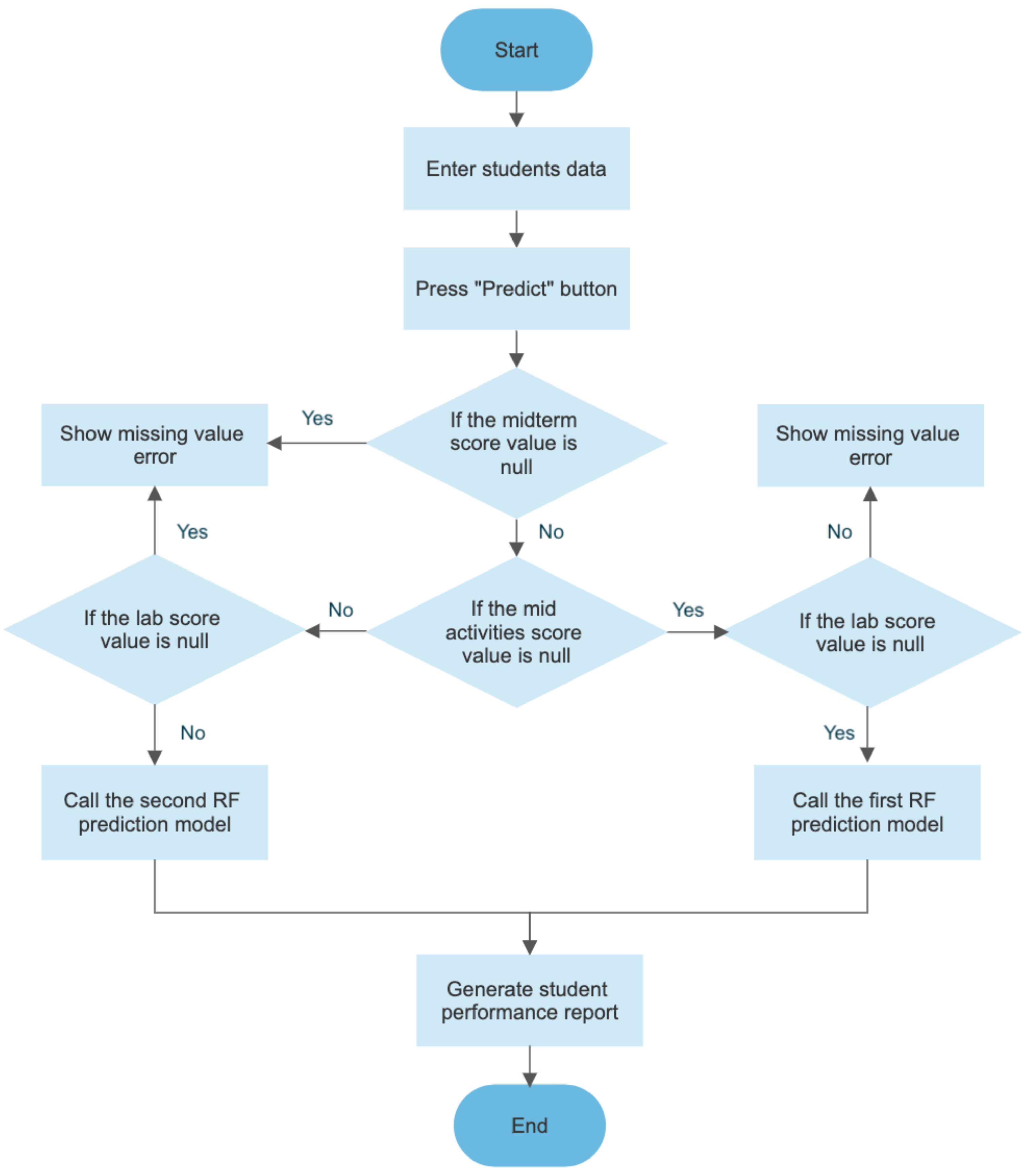
This simple web app is a tangible example of deployment. In a larger industrial setting, deployment can be more complex, involving containerization with Docker, deployment to cloud services (like AWS or Google Cloud), and setting up robust monitoring. The flowchart below shows a more realistic internal logic for a deployed system, where it first validates the input data before calling one of two different models.
Finally, deployment is not the end. Once a model is live, it must be monitored for performance degradation (a concept called "model drift") and periodically retrained on new data to keep it accurate. This continuous cycle is a core part of MLOps (Machine Learning Operations).
Conclusion
In this lesson, we completed our tour of the machine learning project lifecycle. We took our prepared data and moved through the final, crucial stages of bringing a model to life.
Key Takeaways:
- Model Training is the process of an algorithm learning patterns from the training data. The output is a trained model file.
- Model Evaluation is the critical step of testing the model on unseen data to get an honest measure of its performance and avoid overfitting.
- The question "How good is the model?" is answered with quantitative metrics. For regression problems like ours, we use RMSE, MAE, and R-squared to measure prediction error. For classification problems, we use metrics like Precision and Recall.
- Deployment is the process of integrating the best-performing model into a live application so it can make predictions on new, real-world data.
We have now covered the end-to-end workflow of a traditional machine learning project. In our next lesson, we will pivot to explore a specific, highly powerful subfield of machine learning that has driven many of the recent breakthroughs in AI: Deep Learning. We will introduce the fundamental building block of deep learning—the artificial neural network.