Big O Notation: Analyzing Algorithm Complexity

1. What is Big O Notation?

At its core, Big O notation is a way to describe an algorithm's performance as the size of the input, which we'll call $n$, gets very large. It doesn't measure the exact runtime in seconds, which can vary based on the computer's hardware. Instead, it measures the growth rate of the number of operations.

In interviews, we're typically concerned with two things:

1. Time Complexity: How does the runtime of an algorithm grow as the input size $n$ increases?
2. Space Complexity: How does the amount of extra memory the algorithm needs grow as the input size $n$ increases?

Crucially, Big O focuses on the worst-case scenario. This gives us an upper bound on performance, ensuring we know the maximum resources our algorithm might consume. Given your mathematics background, you can think of this as being similar to finding the dominant term in a polynomial to understand its end behavior as $n\to \infty$.

To get a quick, interview-focused overview of Big O, let's start with a video.

As the video explains, Big O simplifies complexity by focusing on the part of the expression that grows the fastest. An algorithm with $2n+10$ operations and one with $0.5n-2$ operations are both considered to have a linear growth rate, which we denote as $O(n)$.

2. Common Complexity Classes

Algorithms are categorized into different complexity classes based on their growth rates. Let's explore the most common ones you'll encounter, from most efficient to least efficient.

The following video provides an excellent tour of these classes with examples you'd see in coding problems.

To visualize the dramatic difference in these growth rates, take a look at this graph. Notice how quickly functions like $O(2^n)$ and $O(n!)$ become computationally infeasible, even for small inputs.

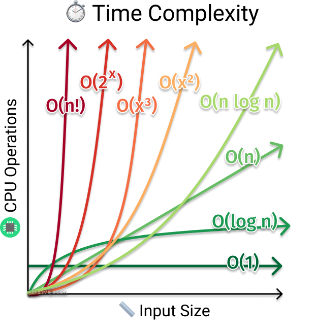
Here is a handy "cheat sheet" that summarizes the common Big O notations with examples. This is a great reference to have.

3. How to Analyze Your Code

Now for the most important part: applying this knowledge to analyze code. The process can be broken down into a few simple rules.

Rules for Calculating Time Complexity

1. Drop Constants: An algorithm that takes $2n$ steps is simplified to $O(n)$. We care about the overall growth rate, not the exact multiplier.
2. Drop Lower-Order Terms: An algorithm that takes $n^2+n$ steps is simplified to $O(n^2)$. For large $n$, the $n^2$ term dominates and makes the $n$ term insignificant.
3. Sequential Statements (Adding): If you have two loops that run one after the other, you add their complexities. For example, a loop that runs $n$ times followed by a loop that runs $m$ times is $O(n+m)$. If they both run $n$ times, it's $O(n+n)=O(2n)\to O(n)$.
4. Nested Statements (Multiplying): If you have a loop inside another loop, you multiply their complexities. A loop that runs $n$ times with another $n$-time loop inside it is $O(n\times n)=O(n^2)$.

This next resource provides a more detailed, step-by-step guide to analysis.

A Note on Space Complexity

Space complexity analysis follows similar rules. We measure the additional space (or auxiliary space) used by the algorithm.

• $O(1)$ Space: The algorithm uses a fixed amount of memory, regardless of input size (e.g., a few variables to store a sum or counters). This is also called an in-place algorithm.
• $O(n)$ Space: The memory usage grows linearly with the input size. This often happens when you create a new data structure (like an array or hash set) that stores a copy of the input or some derivative of it.
• $O(n)$ Space (Recursion): For recursive functions, space is consumed by the call stack. A function that recurses $n$ levels deep will typically use $O(n)$ space.

def find_sum_and_product(numbers):
    sum_val = 0
    product_val = 1
    
    for num in numbers:
        sum_val += num
        
    for num in numbers:
        product_val *= num
        
    print(f"Sum: {sum_val}, Product: {product_val}")

4. Putting It All Together with Examples

Let's look at a few more examples to solidify your understanding. The key is to break down the code into its constituent parts—loops, function calls, and memory allocations—and apply the rules we just discussed.

def print_all_pairs(items):
    for item1 in items:
        for item2 in items:
            print(f"({item1}, {item2})")

def fibonacci(n):
    if n <= 1:
        return n
    return fibonacci(n - 1) + fibonacci(n - 2)

Conclusion

Great work today! You've covered the essential concepts of algorithmic complexity analysis, which will be your guide for the rest of this course.

Here are the key takeaways:

• Big O Notation describes the worst-case growth rate of an algorithm's time or space usage as the input size $n$ grows.
• We simplify Big O expressions by dropping constants and lower-order terms to focus on the dominant factor.
• Common complexity classes, in order of efficiency, include $O(1)$, $O(\log n)$, $O(n)$, $O(n\log n)$, $O(n^2)$, and $O(2^n)$. Knowing which category your algorithm falls into is crucial.
• Analyzing code involves identifying sequential blocks (add complexities) and nested blocks (multiply complexities).
• Space complexity measures extra memory used, including the recursion call stack.

In our next lesson, we will dive into our first problem-solving pattern: array and string traversal. You'll immediately apply what you learned today to analyze the efficiency of algorithms that iterate through data collections.