Classical Probability

The Classical Definition: A Ratio of Counts

The classical approach to probability, developed from analyzing games of chance, is elegant in its simplicity. It defines the probability of an event as the ratio of the number of outcomes that constitute the event to the total number of possible outcomes in the sample space.

This is often expressed as:

Given our work with set theory, we can state this more formally. If $S$ is the sample space and $A$ is an event, the probability of $A$ is:

where $|A|$ denotes the cardinality (the number of elements) of the set $A$.

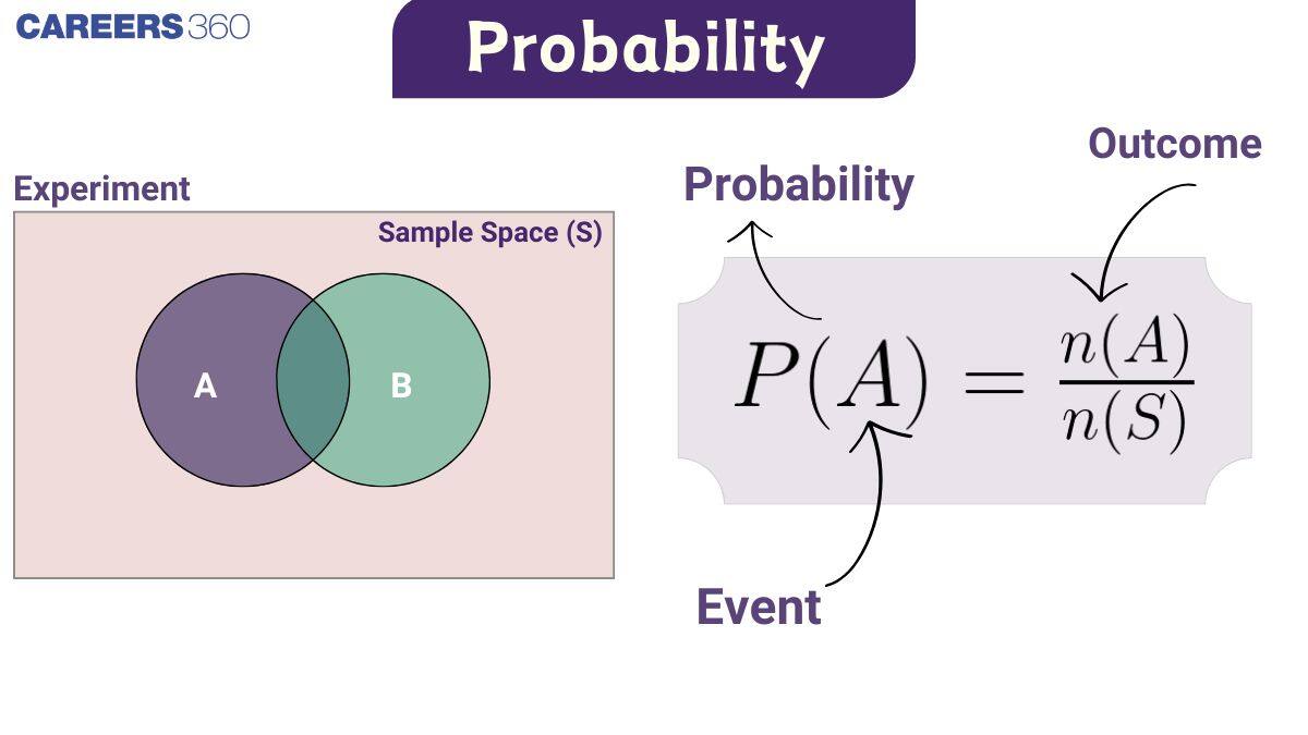
This definition has one crucial prerequisite: all elementary outcomes in the sample space must be equally likely. A fair coin, a balanced die, or a well-shuffled deck of cards are all physical systems designed to satisfy this condition.

Let's ground this with a formal definition from a set of lecture notes on probability.

From Formula to Calculation

With the definition in hand, let's apply it. The process is a direct follow-on from our last lesson:

1. Identify the random experiment.
2. Enumerate all outcomes to define the sample space, $S$, and find its size, $|S|$.
3. Identify the outcomes corresponding to the event of interest, $A$, and find its size, $|A|$.
4. Calculate the ratio $P(A)=|A|/|S|$.

The following video walks through this process with several clear examples, including rolling a die, picking cherries from a bag, and drawing a card from a deck.

A More Involved Example: Rolling Two Dice

Let's apply this to a more complex experiment we analyzed in the previous lesson: rolling two six-sided dice. As we established, the sample space consists of 36 equally likely ordered pairs, from (1, 1) to (6, 6). So, $|S|=36$.

Now, let's calculate the probability of a few events:

• Event A: The sum of the dice is 7.
  The outcomes that satisfy this event are $A=\{(1,6),(2,5),(3,4),(4,3),(5,2),(6,1)\}$.
  The size of the event set is $|A|=6$.
  Therefore, the probability is $P(A)=\frac{|A|}{|S|}=\frac{6}{36}=\frac{1}{6}$.

• Event B: Both dice show the same number (doubles).
  The outcomes are $B=\{(1,1),(2,2),(3,3),(4,4),(5,5),(6,6)\}$.
  The size of the event set is $|B|=6$.
  The probability is $P(B)=\frac{|B|}{|S|}=\frac{6}{36}=\frac{1}{6}$.

The following reading walks through a similar example from the casino game of craps, showing how to systematically identify the winning outcomes and calculate the probability.

The Principle of Indifference

The condition that outcomes must be "equally likely" or "equally possible" is the most important constraint of the classical model. But what does it mean? The 18th-century mathematician Pierre-Simon Laplace articulated this with what is now called the Principle of Indifference: if we have no reason to believe one outcome is more probable than another, we should assign them equal probabilities.

This principle works perfectly for idealized systems like fair dice, where physical symmetry provides a strong reason to assume each face is equally likely to land up. However, it also highlights the limits of this interpretation. We cannot use it to determine the probability that a biased coin will land heads, or the probability of rain tomorrow, as the outcomes are not symmetrical or equally likely.

The video below discusses this core assumption and its philosophical underpinnings.

From a computer science perspective, this principle is implicitly used in many algorithms. When you use a random number generator to select an index from an array of size $N$, you assume that each index has a $1/N$ probability of being chosen. This is a direct application of classical probability, predicated on the assumption that your random function generates outcomes with uniform likelihood.

Conclusion

In this lesson, we took the crucial step from describing possibilities to quantifying them. By learning the classical definition of probability, you can now calculate the likelihood of events in a wide range of well-defined scenarios.

Key Takeaways:

• The classical probability of an event $A$ is the ratio of the number of outcomes in $A$ to the total number of outcomes in the sample space $S$.
• The formula is $P(A)=\frac{|A|}{|S|}$.
• This definition is only valid when all elementary outcomes in the sample space are equally likely.
• The Principle of Indifference provides the logical basis for assuming outcomes are equally likely when there is no evidence to the contrary.

We've focused on the probability of single events. But what if we are interested in the probability of event A or event B occurring? In our next lesson, we will explore this question by learning about the addition rule of probability, which allows us to combine probabilities of different events.