Measures of Central Tendency

What is Central Tendency?

Before we dive into calculations, let's clarify the concept. A measure of central tendency is a single value that attempts to describe a set of data by identifying a central position within that set. It provides a concise summary, a single number that represents the "average" or "most typical" observation.

The Scribbr article "Central Tendency" provides a succinct introduction to the three measures we will cover.

Now, let's explore each of these measures in detail, focusing on how to calculate them and, more importantly, what they truly represent.

The Mean: The Arithmetic Average

The mean is what people most commonly refer to as the "average." It is the sum of all values in a dataset divided by the number of values. Given your background in computer science, you'll appreciate the formal notation.

In statistics, we distinguish between a population (the entire group of interest) and a sample (a subset of the population). The calculation is the same, but the notation differs:

• Population Mean ($\mu$): $\mu =\frac{\sum X}{N}$, where $\sum X$ is the sum of all values in the population and $N$ is the number of values in thepopulation.
• Sample Mean ($\bar{x}$): $\bar{x}=\frac{\sum x}{n}$, where $\sum x$ is the sum of all values in the sample and $n$ is the number of values in the sample.

For example, for the dataset {2, 4, 6, 8, 10}, the mean is:

The mean includes every value in its calculation, which makes it comprehensive. However, this property is also its greatest weakness: it is highly sensitive to outliers.

The following video from the codebasics channel uses a brilliant example from a data science perspective to illustrate this exact problem.

As the video showed, the presence of one extremely high income (an outlier) skewed the mean to a value that was not at all representative of the town's general population. This is a critical concept in data analysis. Relying solely on the mean can be misleading.

The Median: The Robust Middle Ground

When our data has outliers or is skewed, the median often provides a better sense of the central value. The median is the middle value in a dataset that has been sorted in ascending order. It is robust because it depends on the position of values, not their magnitude.

To find the median:

1. Sort the data from smallest to largest.
2. If the number of observations ($n$) is odd, the median is the middle value, at position $\frac{n+1}{2}$.
3. If the number of observations ($n$) is even, the median is the average of the two middle values, at positions $\frac{n}{2}$ and $\frac{n}{2}+1$.

Let's see this in practice with the excellent guide from Scribbr.

The true power of the median becomes apparent in data science applications. In the previous lesson, we discussed handling missing data. The median provides a much safer way to impute (fill in) missing numerical values than the mean, precisely because it isn't affected by outliers.

The same codebasics video provides a perfect illustration of this use case.

The Mode: The Most Frequent Occurrence

The final measure of central tendency is the mode. It is simply the value that appears most frequently in a dataset.

• A dataset can have one mode (unimodal), two modes (bimodal), or more (multimodal).
• If all values appear with the same frequency, the dataset has no mode.

The mode is the only measure of central tendency that can be used for categorical data (e.g., "Mexican" food in the video example), but it can also be used for numerical data.

However, the mode has significant limitations, especially with continuous numerical data. It might not be unique, and it might not be representative of the center of the data at all.

The Relationship Between Mean, Median, and Mode

The most insightful analysis comes not from looking at these measures in isolation, but from comparing them. The relationship between the mean, median, and mode reveals the skewness of a dataset's distribution.

• Symmetrical Distribution (e.g., Normal Distribution): The mean, median, and mode are all equal or very close. The data is balanced around the central point.
• Positively Skewed Distribution (Right Skew): There is a long "tail" of high-value outliers. These outliers pull the mean to the right. In this case: Mean > Median > Mode. A classic example is income data, where a few very high earners pull the mean income up.
• Negatively Skewed Distribution (Left Skew): There is a long "tail" of low-value outliers. These pull the mean to the left. In this case: Mean < Median < Mode. An example might be the age of retirement, where most people retire around 65-70, but some retire much earlier, pulling the mean down.

This image provides a perfect visual summary of these relationships.

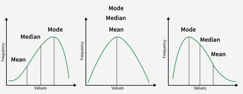
Understanding this relationship is crucial for interpreting your data. If someone reports a mean that is significantly higher than the median, you should immediately suspect the data is positively skewed and that the mean might not be the most representative measure of the "typical" value.

Conclusion

In this lesson, we have taken our first steps in descriptive statistics by learning to calculate and interpret the three measures of central tendency. This is a foundational skill for summarizing any dataset you encounter.

Key Takeaways:

• Mean: The arithmetic average. It is comprehensive but highly sensitive to outliers. Use the notation $\mu$ for a population and $\bar{x}$ for a sample.
• Median: The middle value of a sorted dataset. It is robust to outliers and often a better representation of the center in skewed data. It's also a valuable tool for data preprocessing tasks like imputation.
• Mode: The most frequent value. It is the only measure suitable for categorical data but can be misleading or uninformative for continuous numerical data.
• Interpretation through Comparison: The relative positions of the mean, median, and mode reveal the shape (skewness) of your data's distribution, providing deeper insight than any single measure alone.

You now know how to calculate these three measures and what they tell you about a dataset. In our next lesson, we will build directly on this knowledge to establish clear guidelines for selecting the most appropriate measure of central tendency based on the type of data you have and the shape of its distribution.