Solving Least Squares: Normal Equations & QR Decomposition

1. Method 1: Solving the Normal Equations

In the previous lesson, we used a geometric argument—the orthogonality of the error vector to the column space of A—to derive the normal equations. Given your background in multivariate calculus, you might appreciate an alternative derivation based on optimization.

The least squares problem is to find the vector $\mathbf{x}$ that minimizes the scalar function:
$\varphi (\mathbf{x})=\Vert \mathbf{b}-A\mathbf{x}{\Vert }^2=(\mathbf{b}-A\mathbf{x}{)}^T(\mathbf{b}-A\mathbf{x})$
Expanding this, we get:
$\varphi (\mathbf{x})={\mathbf{b}}^T\mathbf{b}-{\mathbf{b}}^{T}A\mathbf{x}-{\mathbf{x}}^T{A}^T\mathbf{b}+{\mathbf{x}}^T{A}^{T}A\mathbf{x}$
Since ${\mathbf{x}}^T{A}^T\mathbf{b}$ is a scalar, it's equal to its own transpose, $({\mathbf{x}}^T{A}^T\mathbf{b}{)}^T={\mathbf{b}}^{T}A\mathbf{x}$. So we can simplify this to:
$\varphi (\mathbf{x})={\mathbf{b}}^T\mathbf{b}-2{\mathbf{x}}^T{A}^T\mathbf{b}+{\mathbf{x}}^T{A}^{T}A\mathbf{x}$
To find the minimum, we take the gradient with respect to $\mathbf{x}$ and set it to zero. The gradient of this quadratic form is:
$\nabla \varphi (\mathbf{x})=-2A^T\mathbf{b}+2A^{T}A\mathbf{x}$
Setting $\nabla \varphi (\mathbf{x})=0$ gives us $2A^{T}A\mathbf{x}=2A^T\mathbf{b}$, which simplifies to the familiar normal equations:
$A^{T}A\hat{\mathbf{x}}=A^T\mathbf{b}$
This confirms our geometric result using calculus.

A Practical Example

Now that we have the equation, let's see how it's used in practice.

As the video demonstrates, the procedure is:

1. Set up the matrix $A$ and vector $\mathbf{b}$ from your data points and model.
2. Compute the matrix $A^{T}A$ and the vector $A^T\mathbf{b}$.
3. Solve the square linear system $(A^{T}A)\hat{\mathbf{x}}=(A^T\mathbf{b})$ for the parameter vector $\hat{\mathbf{x}}$. You can use any method for solving a linear system, such as Gaussian elimination.

The Caveat: Numerical Instability

The normal equations are elegant, but they have a significant drawback in computational practice. The process of forming $A^{T}A$ can dramatically worsen the conditioning of the problem.

A key result states that the condition number of $A^{T}A$ is the square of the condition number of $A$:
$\text{cond}(A^{T}A)=(\text{cond}(A){)}^2$
If cond(A) is large (meaning the matrix is ill-conditioned), cond(A^T A) will be much larger. This means that small errors in the input data can be greatly amplified in the solution, leading to numerical instability and inaccurate results. This is a critical concern in computer science and numerical analysis.

This motivates the search for a more robust method.

2. Method 2: Solving via QR Decomposition

A better way to solve the least squares problem is to use the QR decomposition, which you'll remember from our module on orthogonality. This method avoids forming $A^{T}A$ altogether.

The Core Idea

Let's start again with the goal of minimizing $\Vert \mathbf{b}-A\mathbf{x}{\Vert }^2$.

1. Decompose the matrix $A$ (assuming it has linearly independent columns) into $A=QR$, where $Q$ is an $m\times n$ matrix with orthonormal columns and $R$ is an $n\times n$ invertible upper triangular matrix.
2. Substitute this into our expression:
   $\Vert \mathbf{b}-QR\mathbf{x}{\Vert }^2$
3. Recall a key property of orthogonal matrices: they preserve the Euclidean norm. That is, $\Vert \mathbf{v}{\Vert }^2=\Vert Q^T\mathbf{v}{\Vert }^2$. We can multiply the vector inside the norm by $Q^T$ without changing the value:
   $\Vert Q^T(\mathbf{b}-QR\mathbf{x}){\Vert }^2=\Vert Q^T\mathbf{b}-Q^{T}QR\mathbf{x}{\Vert }^2$
4. Since $Q$ has orthonormal columns, $Q^{T}Q=I$ (the identity matrix). The expression simplifies beautifully:
   $\Vert Q^T\mathbf{b}-R\mathbf{x}{\Vert }^2$
   Our problem is now to find the $\mathbf{x}$ that minimizes $\Vert Q^T\mathbf{b}-R\mathbf{x}{\Vert }^2$. Since $R$ is invertible, we can make this norm exactly zero by choosing $\mathbf{x}$ such that:
   $R\hat{\mathbf{x}}=Q^T\mathbf{b}$
   This leaves us with a much nicer system to solve. Because $R$ is upper triangular, we can find $\hat{\mathbf{x}}$ easily using back substitution, which is computationally efficient and stable.

The following reading provides a great summary of both the normal equations and this QR approach.

Summary of the QR Method

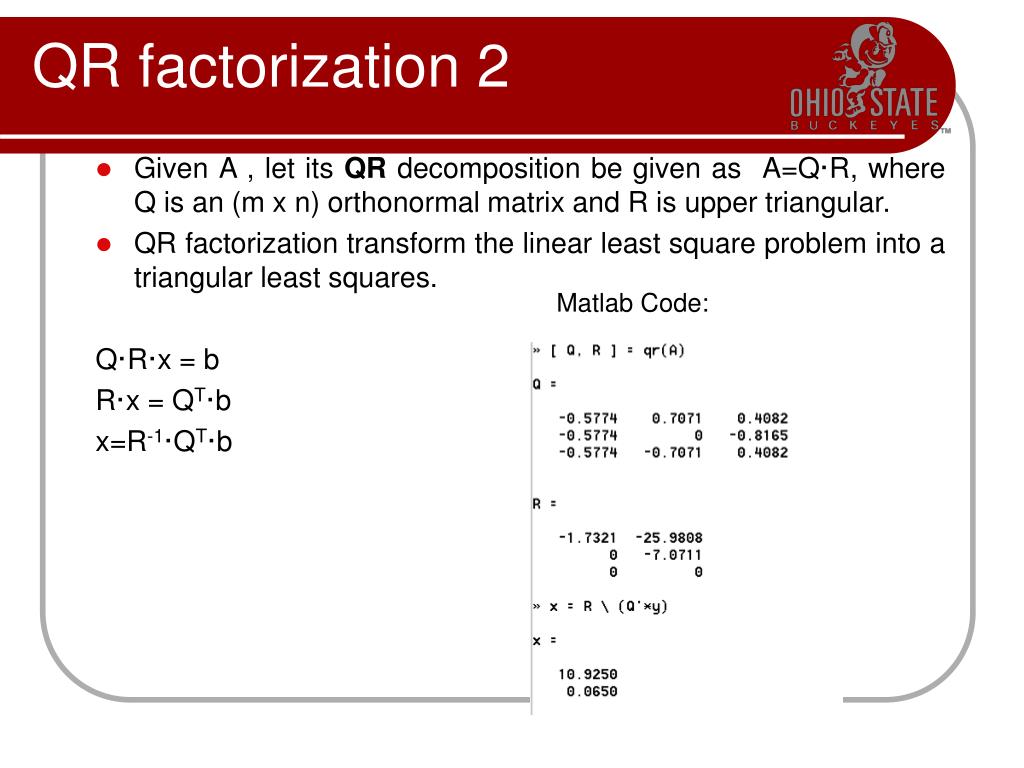
The procedure is as follows:

1. Decompose $A=QR$. (This can be done using the Gram-Schmidt process, which we've studied, or more stable methods like Householder reflections).
2. Compute the vector $\mathbf{c}=Q^T\mathbf{b}$.
3. Solve the upper triangular system $R\hat{\mathbf{x}}=\mathbf{c}$ for $\hat{\mathbf{x}}$ using back substitution.

This process is summarized nicely in the following image, which also includes a code snippet showing how this would be implemented in a language like MATLAB.

Conclusion

Today we explored two powerful techniques for solving the least squares problem. We saw that while the normal equations provide a direct algebraic solution, the QR decomposition offers a more numerically robust and computationally preferred alternative.

Key Takeaways:

• The least squares solution $\hat{\mathbf{x}}$ can be found by solving the normal equations $A^{T}A\hat{\mathbf{x}}=A^T\mathbf{b}$. This method is conceptually straightforward but can be numerically unstable.
• A more stable approach is to use QR decomposition. By factoring $A=QR$, the problem transforms into solving the upper triangular system $R\hat{\mathbf{x}}=Q^T\mathbf{b}$ using back substitution.
• The QR method is generally preferred in practice because it avoids forming the potentially ill-conditioned matrix $A^{T}A$.

Preview of the Next Lesson:

We're not done yet! There is a third, very elegant way to solve the least squares problem that ties together several concepts we've studied, including SVD and matrix inverses. In the next lesson, we will see how to find the least squares solution using the pseudoinverse, which is derived from the Singular Value Decomposition (SVD).