PCA: Maximizing Variance

1. The Challenge: Making Sense of High-Dimensional Data

Imagine you are studying a complex system, like the performance of a deep learning model. You might track dozens or even hundreds of variables: learning rates, layer sizes, activation function types, training times, memory usage, different error metrics, etc. Trying to understand the relationships between all these variables by looking at them one by one is nearly impossible.

This is a common problem in data analysis. We often have datasets with many features (high dimensionality), where:

• Some features might be redundant (e.g., measuring temperature in both Celsius and Fahrenheit).
• The data is often noisy, making it hard to see the underlying patterns.
• The most important relationships might not align with our original measurement axes.

A great way to visualize this problem is with a simple physics example.

As the example illustrates, our goal is to cut through the noise and redundancy to find the true, underlying simplicity in the data. PCA provides a systematic way to do this.

2. The Guiding Principle: Maximizing Variance

So, how can we find the "important" patterns in a cloud of data points? The core idea behind PCA is that the most important directions are those along which the data varies the most.

Imagine you're a whale shark swimming towards a swarm of krill. To eat as many as possible, you'd orient your wide mouth along the direction where the krill are most spread out. PCA does the same thing: it finds the axes along which the data is most spread out.

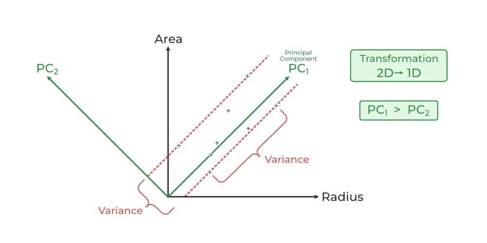
Why is this a good strategy? A direction with high variance is a direction that captures a lot of information about the data. A projection onto a high-variance axis preserves the spread of the data, and therefore the distances between points, much better than a projection onto a low-variance axis.

The following video provides an excellent and concise explanation of this exact point.

The key takeaway is that by prioritizing directions of high variance, we are essentially creating a new coordinate system that is optimally aligned with the structure of our data. The axes of this new system are called principal components.

3. Variance and Covariance: Quantifying Spread and Redundancy

Maximizing variance is about finding the most informative directions. But we also need to handle redundancy. To do this, we need to formalize these ideas with two statistical concepts: variance and covariance.

• Variance: Measures the spread of data along a single dimension. A high variance means the data is spread out. This is what we want to maximize.
• Covariance: Measures how two dimensions vary together. A high positive covariance means that when one variable increases, the other tends to increase as well. A high negative covariance means they have an inverse relationship. A covariance near zero means they are uncorrelated—there's no linear relationship between them. This is what we want to achieve for our new axes.

The following video gives a great visual intuition for covariance and introduces the covariance matrix, which neatly organizes all the variances and covariances for a dataset.

The covariance matrix is the key. For a dataset with $m$ features, it's an $m\times m$ symmetric matrix where:

• The diagonal entries, $C_{ii}$, are the variances of each feature.
• The off-diagonal entries, $C_{ij}$, are the covariances between feature $i$ and feature $j$.

4. The Conceptual Framework of PCA

Now we can combine these ideas to define the conceptual goal of PCA. PCA aims to find a new basis (a new set of coordinate axes) to represent the data, such that in this new representation:

1. Redundancy is eliminated. The new features are uncorrelated, meaning the covariance matrix of the transformed data is diagonal.
2. Information is maximized. The new features (principal components) are ordered by variance, so the first few components capture most of the information in the data.

This is a powerful goal that turns a geometric intuition into a precise algebraic objective. Let's return to the Shlens tutorial to see this framework laid out.

To summarize the key points from the reading:

• We assume that directions with large variance contain interesting dynamics (signal), while directions with low variance are noise.
• We view high covariance between variables as redundancy.
• Therefore, the ideal representation of the data would be in a basis where the covariance matrix is diagonal. The diagonal entries would be the variances of our new basis vectors (the principal components), and the off-diagonal entries (the covariances) would be zero.
• PCA finds this new basis by, in essence, performing a rotation. The first principal component is the direction in space that maximizes variance. The second is the direction that maximizes variance subject to being orthogonal to the first, and so on.

A Crucial Prerequisite: Data Centering

One important practical step is that before computing the covariance matrix and finding principal components, the data must be centered. This means that for each feature, we calculate its mean and subtract it from all data points. This ensures the data cloud is centered at the origin.

Why? Variance and covariance are defined as spread around the mean. If we don't center the data, the first principal component might just point from the origin to the center of the data, which tells us where the data is, but not the direction of its spread. Centering ensures we are only measuring the variance of the data itself.

Conclusion

In this lesson, we built the conceptual framework for Principal Component Analysis. We didn't get into the full computational details, but focused on the intuitive why.

Key Takeaways:

• PCA is a technique to find a more informative representation of high-dimensional data by creating a new set of coordinate axes, the principal components.
• The fundamental principle of PCA is to find directions of maximum variance, as these directions capture the most information and preserve the structure of the data.
• The goal is to find a new basis where the features are uncorrelated. Algebraically, this means finding a basis that diagonalizes the covariance matrix.
• The principal components are orthogonal axes, ordered by the amount of variance they explain. The first PC accounts for the most variance, the second for the next most, and so on.

Preview of the Next Lesson:
We've defined the what and the why. Next, we'll tackle the how. We will formalize the process and see a beautiful connection back to our previous topics: the principal components are nothing more than the eigenvectors of the covariance matrix, or equivalently, the right singular vectors ($V$) of the centered data matrix. This will link PCA directly to SVD and give us a concrete way to compute the components.