Gram-Schmidt Orthonormalization

1. The Core Idea: Purification by Projection

Imagine you have a basis of vectors, but they're "messy"—skewed at various angles. An orthonormal basis is "clean"—all vectors are at 90-degree angles to each other and have a length of 1. The Gram-Schmidt process is an algorithm that "purifies" a messy basis into a clean one, vector by vector.

The key insight is to use orthogonal projection, a concept we've encountered before. For each vector in our original basis, we'll subtract the parts of it that are "contaminated" by the directions of the new, clean vectors we've already built. What remains is the "pure" part, a new vector that is orthogonal to all the previous ones.

Professor Gilbert Strang provides a wonderful intuitive introduction to this idea.

As Professor Strang explained, the process for two vectors, $\{{\mathbf{v}}_1,{\mathbf{v}}_2\}$, works as follows:

1. First vector: We have nothing to make it orthogonal to yet, so we just accept the first vector as is. Let our first new orthogonal vector be ${\mathbf{u}}_1={\mathbf{v}}_1$.
2. Second vector: We "purify" ${\mathbf{v}}_2$ by subtracting its projection onto ${\mathbf{u}}_1$. The result, ${\mathbf{u}}_2$, will be orthogonal to ${\mathbf{u}}_1$. $${\mathbf{u}}_2={\mathbf{v}}_2-{\text{proj}}_{{\mathbf{u}}_1}({\mathbf{v}}_2)={\mathbf{v}}_2-\frac{⟨{\mathbf{v}}_2,{\mathbf{u}}_1⟩}{⟨{\mathbf{u}}_1,{\mathbf{u}}_1⟩}{\mathbf{u}}_1$$

2. The General Algorithm

We can generalize this procedure to any number of vectors. To find the $k$-th orthogonal vector ${\mathbf{u}}_k$, we take the original $k$-th vector ${\mathbf{v}}_k$ and subtract its projections onto all the previously constructed orthogonal vectors ${\mathbf{u}}_1,{\mathbf{u}}_2,\dots ,{\mathbf{u}}_{k-1}$.

The image below illustrates this for finding the second and third orthogonal vectors.

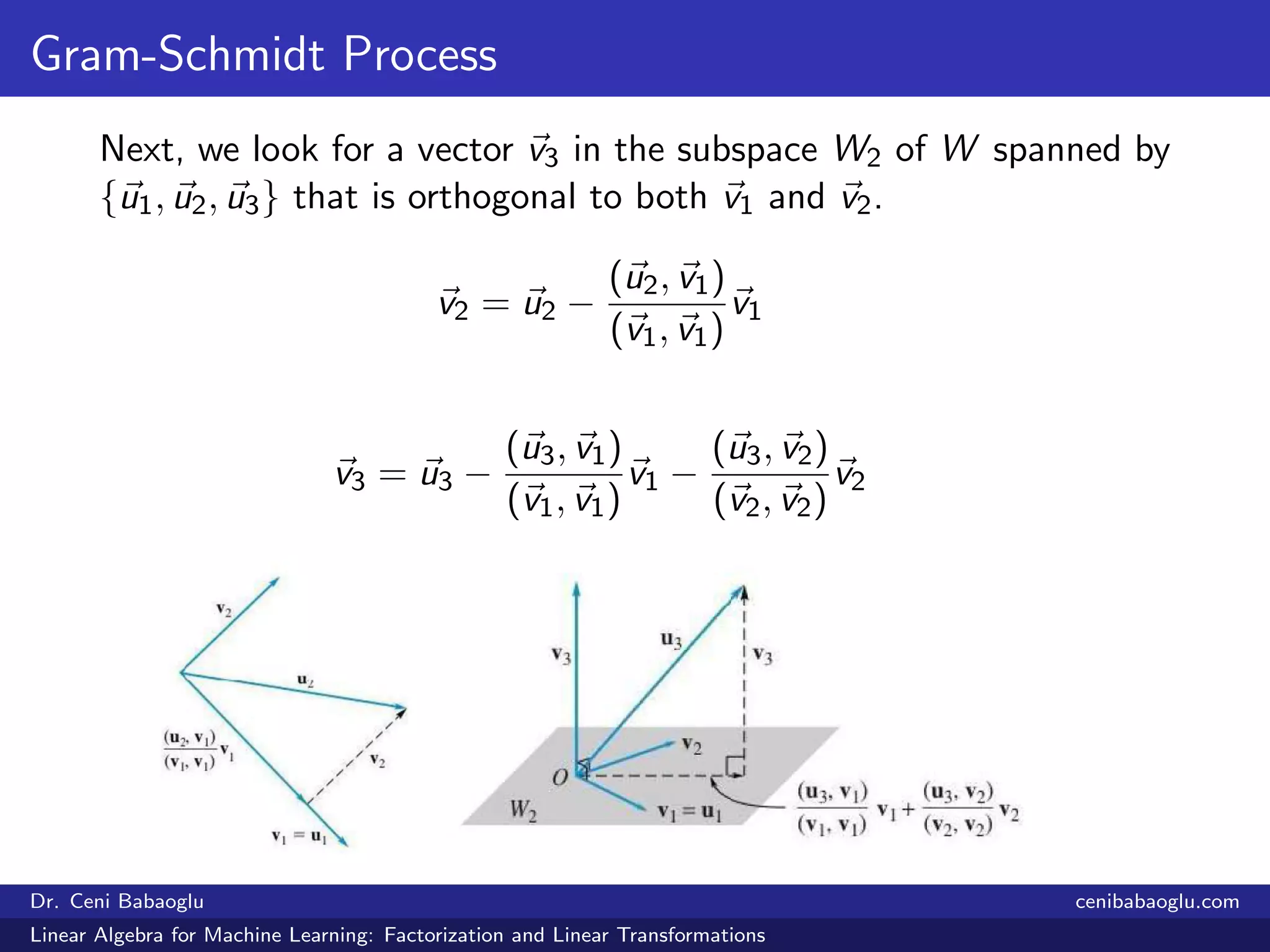
This leads to the general formula for constructing an orthogonal basis $\{{\mathbf{u}}_1,\dots ,{\mathbf{u}}_n\}$ from an initial basis $\{{\mathbf{v}}_1,\dots ,{\mathbf{v}}_n\}$:

• ${\mathbf{u}}_1={\mathbf{v}}_1$
• ${\mathbf{u}}_2={\mathbf{v}}_2-\frac{⟨{\mathbf{v}}_2,{\mathbf{u}}_1⟩}{⟨{\mathbf{u}}_1,{\mathbf{u}}_1⟩}{\mathbf{u}}_1$
• ${\mathbf{u}}_3={\mathbf{v}}_3-\frac{⟨{\mathbf{v}}_3,{\mathbf{u}}_1⟩}{⟨{\mathbf{u}}_1,{\mathbf{u}}_1⟩}{\mathbf{u}}_1-\frac{⟨{\mathbf{v}}_3,{\mathbf{u}}_2⟩}{⟨{\mathbf{u}}_2,{\mathbf{u}}_2⟩}{\mathbf{u}}_2$
• ...
• ${\mathbf{u}}_k={\mathbf{v}}_k-{\sum }_{i=1}^{k-1}\frac{⟨{\mathbf{v}}_k,{\mathbf{u}}_i⟩}{⟨{\mathbf{u}}_i,{\mathbf{u}}_i⟩}{\mathbf{u}}_i$

From Orthogonal to Orthonormal

Once we have our orthogonal basis $\{{\mathbf{u}}_1,\dots ,{\mathbf{u}}_n\}$, creating an orthonormal basis $\{{\mathbf{q}}_1,\dots ,{\mathbf{q}}_n\}$ is simple. We just normalize each vector by dividing it by its norm (length). This was "Schmidt's contribution" in Professor Strang's telling.

3. A Complete Worked Example

The algorithm can look intimidating, but it's a straightforward computation. The following video walks through a full example in ${\mathbb{R}}^3$ and clearly lays out all the steps.

Let's recap the complete process:
Given a basis $\{{\mathbf{v}}_1,\dots ,{\mathbf{v}}_n\}$:

1. Orthogonalize: For $k=1,\dots ,n$, compute ${\mathbf{u}}_k={\mathbf{v}}_k-{\sum }_{i=1}^{k-1}{\text{proj}}_{{\mathbf{u}}_i}({\mathbf{v}}_k)$.
2. Normalize: For $k=1,\dots ,n$, compute ${\mathbf{q}}_k={\mathbf{u}}_k/\Vert {\mathbf{u}}_k\Vert$.

The resulting set $\{{\mathbf{q}}_1,\dots ,{\mathbf{q}}_n\}$ is an orthonormal basis for the same space spanned by the original vectors.

4. Practical Implications for Computer Science

For a computer science student, it's crucial to know that while the "Classical" Gram-Schmidt (CGS) process we've just learned is mathematically sound, it suffers from a major drawback in practice: numerical instability. When implemented on a computer, floating-point rounding errors can accumulate, causing the resulting vectors to lose their orthogonality.

A slightly rearranged version, the Modified Gram-Schmidt (MGS) process, is mathematically equivalent but far more robust to these errors. In MGS, after a vector ${\mathbf{q}}_k$ is produced, its components are immediately removed from all subsequent vectors ${\mathbf{v}}_{k+1},{\mathbf{v}}_{k+2},\dots$. This "pay as you go" approach prevents errors from accumulating.

The following notes provide a more rigorous look at Gram-Schmidt, including a striking example that shows how CGS can fail in practice while MGS succeeds. This is a perfect illustration of why numerical linear algebra is a deep field.

The Gram-Schmidt process is also the theoretical foundation for QR factorization, a cornerstone of numerical computing. It states that any matrix $A$ with linearly independent columns can be factored into $A=QR$, where:

• Q is a matrix with orthonormal columns (the basis vectors we just made!).
• R is an upper-triangular matrix that stores the "recipe" of the projections.

This decomposition is used everywhere, from solving linear systems to the algorithms inside deep learning libraries. In practice, you would use a library function like np.linalg.qr in Python, which typically uses a stable variant of Gram-Schmidt or other, even more robust methods.

Conclusion

Today, we've added a powerful constructive tool to our linear algebra toolkit. The Gram-Schmidt process provides a concrete algorithm for turning any basis into a much more convenient orthonormal basis.

Key Takeaways:

• The Gram-Schmidt process builds an orthonormal basis by sequentially orthogonalizing and then normalizing vectors.
• The core step is projection: to make a vector ${\mathbf{v}}_k$ orthogonal to the existing set $\{{\mathbf{u}}_1,\dots ,{\mathbf{u}}_{k-1}\}$, you subtract the projection of ${\mathbf{v}}_k$ onto each of those vectors.
• The classical version of the algorithm is numerically unstable; the Modified Gram-Schmidt process is used in practice for better accuracy.
• This process is the theoretical basis for QR decomposition, a fundamental tool in computational science.

Preview of the Next Lesson:

The Gram-Schmidt process used projection as a building block to orthogonalize a set of vectors. In the next lesson, we will focus directly on the orthogonal projection of a single vector onto an entire subspace. This will generalize our work from today and give us the primary tool needed to solve "unsolvable" systems of linear equations, leading directly to the concept of least squares approximation—a fundamental technique in data analysis and machine learning.